Personalized Thermal Comfort Forecasting for Smart Buildings via

Locally Weighted Regression with Adaptive Bandwidth

Carlo Manna, Nic Wilson and Kenneth N. Brown

Cork Constraint Computation Centre(4C), Dept. Computer Science, University College Cork, Cork, Ireland

Keywords:

Machine Learning, Smart Buildings, Thermal Comfort.

Abstract:

A personalized thermal comfort prediction method is proposed for use in combination with smart controls

for building automation. Occupant thermal comfort is traditionally measured and predicted by the Predicted

Mean Vote (PMV) metric, which is based on extensive ﬁeld trials linking reported comfort levels with the

various factors. However, PMV is a statistical measure applying to large populations, and the actual thermal

comfort could be signiﬁcantly different from the predicted value for small groups of people. Moreover it may

be hard to use for a real-time controller due to the number of sensor readings needed. In the present paper,

we propose Robust Locally Weighted Regression with Adaptive Bandwidth (LRAB), a kernel based method,

to learn individual occupant thermal comfort based on historical reports. Using publicly available datasets,

we demonstrate that this technique is signiﬁcantly more accurate in predicting individual comfort than PMV

and other kernel methods. Therefore, is a promising technique to be used as input to adpative HVAC control

systems.

1 INTRODUCTION

Energy-efﬁciency for buildings is currently a topic

of major interest, especially with increasing energy

costs. In particular, the HVAC (heating ventilation

and air conditioning) system, which ensures thermal

comfort conditions in ofﬁces (during both wintertime

and summer), on the other is one of the main energy

consumers in a building. For this reason, accurately

predicting comfort levels for the occupants can en-

able one to avoid unnecessary heating or cooling, and

thus improve the energy efﬁciency of the HVAC sys-

tems. A number of thermal comfort indices (indica-

tors of human comfort) have been studied for the de-

sign of HVAC systems (Fanger, 1972; Gagge et al.,

1986), the most widely used of which is the Predicted

Mean Vote (PMV) index, which was developed by

Fanger (Fanger, 1972). However, to ﬁnd appropri-

ate set-point temperatures with the PMV standard,

the designer has to make assumptions about cloth-

ing and activity of occupants. Moreover, for small

groups of people within a single room or zone in a

building, PMV may not perform an accurate predic-

tion as pointed out in (Kumar and Mahdavi, 2001) and

in (Humphreys and Nicol, 2000). To address these is-

sues, newer standards such as the recently accepted

revisions to ASHRAE Standard 55, that include a

new adaptive comfort standard (ACS) (de Dear and

Brager, 2002), suggests an alternative (or a comple-

mentary) theory of thermal perception based on the

psychological dimension of adaptation, which may be

particularly important in contexts where people’s in-

teractions with the environment (i.e. personal thermal

control), or diverse thermal experiences, may alter

their expectations, and thus, their thermal sensation

and satisfaction. In particular, the level of comfort

perceivedby each individual also depends on their de-

gree of adaptation to the context and to the environ-

mental changes, and therefore the speciﬁcity of each

individual should be taken into account to learn and

predict comfort satisfaction.

For these reasons, in the present paper, we pro-

pose an alternative approach tailored to individual oc-

cupants, which relies on historical data on individ-

ual responses to internal environment conditions. We

propose Robust Locally Weighted Regression (Cleve-

land, 1979) with an Adaptive Bandwidth (LRAB), a

kernel based method, to learn, automatically, the com-

fort model of each user based on their history. We ap-

plied this method using up to three input variables (in-

side air temperature, humidity and mean radiant tem-

perature) which do not require expensive sensors and

are easy to measure. Finally, we compare the pro-

posed method with both PMV and a standard kernel

Manna C., Wilson N. and Brown K..

Personalized Thermal Comfort Forecasting for Smart Buildings via Locally Weighted Regression with Adaptive Bandwidth.

DOI: 10.5220/0004375100320040

In Proceedings of the 2nd International Conference on Smart Grids and Green IT Systems (SMARTGREENS-2013), pages 32-40

ISBN: 978-989-8565-55-6

 2013 SCITEPRESS (Science and Technology Publications, Lda.)

method, the Nadaraya-Watson kernel method (with

different kernel functions), using publicly available

datasets (ASHRAE, RP-884). Our experimental re-

sults show that LRAB outperforms both the PMV and

the Nadaraya-Watson kernel method in predicting in-

dividual comfort, and hence it is a promising tech-

nique to be used as an input to the heating/cooling

control systems in an ofﬁce environment.

The paper is organised as follows: in the next sec-

tion, some backgroundon PMV and on alternative ex-

isting techniques are reported. Then, in section 2, the

Nadaraya-Watson kernel and the proposed method are

described, while in the section 3, the experimental re-

sults using a public dataset are shown. Finally, in sec-

tion 4, conclusions and future directions are reported.

1.1 Previous Research

Many methods have been proposed for comfort eval-

uation and prediction; a comprehensive overview is

given in (Olesen, 2004). However, as stated in the

previous section, the most widely used of these is the

PMV index, which has been an international standard

since the 1980s (ASHRAE, 2010), (ISO, 1994). The

conventional PMV model predicts the mean thermal

sensation vote on a standard scale for a large group

of people in a given indoor climate. Like the other

methods described in (Olesen, 2004), it is a function

of two human variables and four environmental vari-

ables, i.e. clothing insulation worn by the occupants,

human activity, air temperature, air relative humidity,

air velocity and mean radiant temperature. The values

of the PMV index have a range from -3 to +3, which

corresponds to an occupant’s thermal sensation from

cold to hot, with the zero value of PMV meaning neu-

tral. As mentioned above, PMV is not just an index

to measure the comfort level, but it is also, and espe-

cially, a model to predict the thermal sensation given

the indoor environmental conditions. It has been val-

idated by many studies, both in climate chambers and

in buildings (Busch, 1992; Yang and Zhang, 2008).

The standard approach to comfort-based control in-

volves regulating the internal environment variables

to ensure a PMV value of zero (Shukor et al., 2007;

Yang and Su, 1997; Freire et al., 2008).

1.1.1 Predicted Mean Vote and its Alternative

Versions

Although PMV can be succesfully used in a design

phase (both for houses and buildings), it has some

drawbacks when used for HVAC controllers. Firstly,

it requires a substantial amount of environmentaldata.

For a controller in real-time this information is only

accessible via sensors. However some measurements,

such as air velocity, require costly sensors, while,

there are no sensors for variables such as clothing and

activity level. Secondly, PMV is a statistical measure

which assumes a large number of people experienc-

ing the same conditions. For small groups of peo-

ple within a single room or zone in a building, how-

ever, PMV may not be an accurate measure. (Ku-

mar and Mahdavi, 2001) analysed the discrepancy

between predicted mean vote proposed in (Fanger,

1972) and observed values based on a meta-analysis

of the ﬁeld studies database made available under

ASHRAE RP-884 and ﬁnally proposing a framework

to adjust the value of thermal comfort indices (a

modiﬁed PMV). The large ﬁeld studies on thermal

comfort described in (Humphreys and Nicol, 2002),

(de Dear and Schiller Brager, 2001) and (Humphreys

and Nicol, 2000), have shown that PMV does not give

correct predictions for all environments. (de Dear

and Schiller Brager, 2001) found PMV to be unbi-

ased when used to predict the preferred operativetem-

perature in the air conditioned buildings. PMV did,

however, overestimate the subjective warmth sensa-

tions of people in warm naturally ventilated buildings.

(Humphreys and Nicol, 2000) showed that PMV was

less closely correlated with the comfort votes than

were the air temperature or the mean radiant temper-

ature, and that the effects of errors in the measure-

ment of PMV were not negligible. Finally the work

in (Humphreys and Nicol, 2002) also showed that the

discrepancy between PMV and the mean comfort vote

was related to the mean temperature of the location.

In addition to the relative inaccuracy, the PMV model

is a nonlinear relation, and it requires iteratively com-

puting the root of a nonlinear equation, which may

take a long computation time. Therefore, a number

of authors have proposed alternative methods of cal-

culation to the main one proposed in (Fanger, 1972).

Fanger and (ISO, 1994) suggest using tables to de-

termine the PMV values of various combinations be-

tween the six thermal variables. (Sherman, 1985) pro-

posed a simpliﬁed model to estimate the PMV value

without any iteration step, by linearizing the radia-

tion exchange term in Fanger’s model. This study in-

dicated that the simpliﬁed model was only accurate

when the occupants are close to being comfortable.

(Federspiel and Asada, 1992) proposed a thermal sen-

sation index, which is a modiﬁed form of Fanger’s

model. They assumed that the radiative exchange and

the heat transfer coefﬁcient are linear, and they also

assumed that the clothing insulation and heat gener-

ation rate of human activity are constant. They then

derived a thermal sensation index that is an explicit

function of the four environmental variables. How-

ever, as the authors said, the simpliﬁcation of Fanger’s

PersonalizedThermalComfortForecastingforSmartBuildingsviaLocallyWeightedRegressionwithAdaptiveBandwidth

PMV model results in signiﬁcant error when the as-

sumptions are not respected. On the other hand, in

(Bingxin et al., 2011) and (Atthajariyakul and Leep-

hakpreeda, 2005) different approaches have been pro-

posed in order to compute PMV avoiding the difﬁcult

iterative calculation. The former proposes a Genetic

Algorithm Back Propagation neural network to learn

user comfort based both on historical data and real-

time environmental measurements. The latter pro-

poses a neural network applied to the iterative part of

the PMV model that, after a learning phase, based on

historical data, avoids the evaluation of such iterative

calculation in real-time.

1.1.2 Beyond the PMV

Recent trends in the study of thermal environment

conditions for human occupants are reported in the

recently accepted revisions to ASHRAE Standard

55, which includes a new adaptive comfort standard

(ACS). According to (de Dear and Brager, 2002) this

adaptive model could be an alternative (or a comple-

mentary) theory of thermal perception. The funda-

mental assumption of this alternative point of view

states that factors beyond fundamental physics and

physiology play an important role in building occu-

pants’ expectations and thermal preferences. PMV

does take into account the heat balance model with

environmental and personal factors, and is able to ac-

count for some degrees of behavioral adaptation such

as changing one’s clothing or adjusting local air ve-

locity.

However, it does not take into account the possi-

ble adaptation of an individual as a result from his/her

interaction with the environment (i.e. personal ther-

mal control), which, in turn, may alter his/her expec-

tations, and thus, their thermal sensation and satis-

faction. In particular, the level of comfort perceived

by each individual also depends on their degree of

adaptation to the context and to the environmental

changes, and therefore the speciﬁcity of each individ-

ual should be taken into account to learn and predict

comfort satisfaction.

For this reason, some authors have proposed tech-

niques based on learning the perception of comfort by

individuals. For example, in (Feldmeier and Paradiso,

2010) the author proposes a system able to learn in-

dividual thermal preferences using a Nearest Neigh-

bor Classiﬁer, taking into account only four variables

(air temperature, humidity, clothing insulation and

human activity), acquired by means of wearable sen-

sors. In (Schumann et al., 2010), a Nearest Neighbor

Classiﬁcation-like method was implemented in order

to learn individual user preferences based on histori-

cal data, using only one variable (air temperature). On

other hand in (Daum et al., 2011) the authors propose

a personalized measure of thermal comfort based on

logistic regression to convert user votes to a probabil-

ity of comfort.

In this study we consider such alternative and

more practical approaches to predicting thermal com-

fort through the automatic learning of the comfort

model of each user based on his/her historical records.

We apply the Robust Locally Weighted Regression

technique (Cleveland, 1979) with an Adaptive Band-

width (LRAB), one of the family of statistical pat-

tern recognition methods. Non-parametric regres-

sion methods, or kernel-based methods, are well es-

tablished methods in statistical pattern recognition

(Hastie et al., 2003). These methods do not need any

speciﬁc prior relation among data. Hence, there are

no parameter estimates in non-parametric regression.

Instead, to forecast, these methods retain the data

and search through them for past similar cases. This

strength makes non-parametric regression a powerful

method due to its ﬂexible adaptation in a wide vari-

ety of situations. The Robust Locally Weighted Re-

gression is one of a number of nonparametric regres-

sions. It ﬁts data by local polynomial regression and

joins them together. The ﬁrst version of this method

was ﬁrst introduced by Cleveland (Cleveland, 1979),

and it was further developed for multivariate models

in (Cleveland and Devlin, 1988).

2 KERNEL METHODS

In this section we describe a class of techniques used

throughout this paper, which achieve ﬂexibility in es-

timating the regression function f (X) over domain

ℜ

by ﬁtting a different but simple model separately

at each query point x in ℜ

. This is done by using

only those observations close to the target point x to

ﬁt the simple model, and in such a way that the result-

ing estimated function

[

f(X) is smooth. This local-

ization is achieved by means of a weighting function

kernel K

(x,x

), assigning a weight to x

based on its

distance from x. The kernels K

are generally char-

acterized by a parameter λ that is related to the width

of the neighborhood (i.e. kernel bandwidth). In the

next section we ﬁrst describe the Nadaraya-Watson

kernel-weighted average, then in 2.2 the Robust Lo-

cally Weighted Regression and, ﬁnally, in 2.3 the pro-

posed approach to select the kernel bandwidth λ.

2.1 Nadaraya-Watson Kernel Method

Let (x

) denote a response, y

, to a recorded value

∈ ℜ

, for i = 1,. .., n. In this paper x

denotes the

SMARTGREENS2013-2ndInternationalConferenceonSmartGridsandGreenITSystems

environmental variables (inside air temperature, hu-

midity etc.) and the response y

represents the satis-

faction degree (real-valued from −3 to +3) that the

user has given in response to the condition x

, and

then stored in a database. The aim is to assess the

response ˆy =

f(x) (i.e. predict the degree of satisfac-

tion) for any new input value x. The approach aims to

estimate a local mean around x, giving all the points

in the neighborhood different weights. In particular,

we can assign weights that die off smoothly with dis-

tance to the target point. In the Nadaraya-Watson ker-

nel method (Bishop, 2006) the resulting estimated re-

sponse ˆy is:

f(x) =

∑

i=1

(x,x

∑

i=1

(x,x

)

(1)

There are many kernel functions K

proposed in

the literature. In this paper we used three different

kernel functions among the most used and which gen-

erally lead to satisfactory results.

2.1.1 Epanechnikov Quadratic Kernel

The Epanechnikov quadratic kernel is deﬁned as fol-

low:

(x,x

) = D



|x− x



(2)

with

D(σ) =

(

(1− σ

) if |σ| ≤ 1,

0 otherwise.

The smoothing parameter λ, which determines the

width of the local neighborhood, has to be chosen.

Large λ implies lower variance (it takes into account

more observation points), but higher bias (it assumes

the true function is almost constant inside the win-

dow).

2.1.2 Tricube Kernel

The tricube kernel is another popular compact kernel.

It is still deﬁned by Equation (2) but with:

D(σ) =

(

(1− |σ|

)

if |σ| ≤ 1,

0 otherwise.

This is ﬂatter on the top than Epanechnikov kernel

and is differentiable at the boundary.

2.1.3 Gaussian Kernel

The Gaussian kernel is a popular non-compact kernel.

It consists in the Gaussian density function D(σ) =

ψ(σ), which is centered in the query point x, and with

the standard deviation playing the role of the window

size.

2.2 Robust Locally Weighted

Regression with Adaptive

Bandwidth

This method is based on the work in (Cleveland,

1979). In the following, we will only describe the

proposed LRAB method, while for a more general

description of the robust locally weighted regression,

the readers should refer to the work in (Cleveland,

1979). Before giving precise details on the LRAB

procedure, we attempt to explain the basic idea of

the method. Recall that (x

) denotes a response,

, to a recorded value x

∈ ℜ

, for i = 1, ... ,n, stored

in a database.The aim is still to assess the response

ˆy =

f(x) for a new input value x. Let b(x) be a vec-

tor of polynomial terms of degree d. For example,

if we have a linear regression (d = 1) in two vari-

ables (p = 2), we have b(x) = (1,x

), or if we a

quadratic regression (d = 2) in two variables (p = 2),

we have b(x) = (1,x

), At each query point

x ∈ ℜ

, the aim is to solve:

min

β(x)

∑

i=1

(x,x

)(y

− b(x

)

β(x))

(3)

to ﬁnd the estimated function

f(x) = b(x)

β(x). The

kernel will be a function such as those deﬁned in sec-

tion 2.1. This procedure computes the initial ﬁtted

values. Anyway, in the real-world, some recorded

values (x

) could be affected by noise or be un-

reliable. The above procedure doesn’t itself elimi-

nate such values. The general idea to do this, is to

strengthen the above preliminary estimation, assign-

ing a different weight ψ

to each pairs (x

) based

on the residual ( ˆy

− y

) (the larger the residual, the

smaller the associated weight). Then, the equation

(3) is computed replacing K

with ψ

∗ K

. This is

an iterative procedure. In this way, and generally af-

ter few iterations, the contribution of some eventually

noisy points to the regression is decreased. To achieve

this goal, let us deﬁne the bisquare function:

Γ(ξ) = (1− ξ

)

(4)

for |ξ| < 1; otherwise Γ(ξ) = 0. Then, for a ﬁxed

new entry point x, let:

= ( ˆy

− y

) (5)

be the residuals for i = 1, ..., n, between the origi-

nal points y

and the estimated points ˆy

(i.e. by means

PersonalizedThermalComfortForecastingforSmartBuildingsviaLocallyWeightedRegressionwithAdaptiveBandwidth

5 10 15 20 25 30 35 40 45

−2

Inside air Temperature [Celsius]

User Votes [PMV scale]

0 10 20 30 40 50 60 70 80 90 100

−2

Relative Humidity [%]

User Votes [PMV scale]

0 5 10 15 20 25 30 35 40 45 50

−2

Mean Radiant Temperature [Celsius]

User Votes [PMV scale]

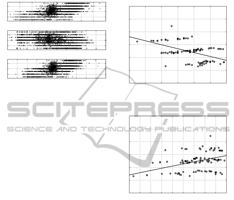
Figure 1: Subset of thermal perceived sensation (in PMV

scale) from users vs inside air temperature, humidity and

mean radiant temperature from database (ASHRAE, RP-

884).

β(x)), and let m be the median of the |ρ

|. As de-

scribed in (Cleveland, 1979), we now choose robust-

ness weights by:

= Γ(ρ

/6m) (6)

At each step of the proposed procedure, the equa-

tion (6) is used to update the weight of the kernel

function in the equation (3) based on the residual ρ

In this way the value of the kernel function in (3) at

each recorded point x

, is decreased (increased) where

the residual value in x

(i.e. ψ

) is too high (too low),

so as to improve the regression for the next step.

2.2.1 Adaptive Bandwidth

In order to choose the bandwidth λ, we ﬁrst needs

to take into account the fact that the density of the

recorded data may be variable. Figure 1 shows a

global view of a subset of ﬁeld data from a public

database (ASHRAE, RP-884), which were used for

our tests. In this ﬁgure, for all three graphs, it shows

the thermal perception from users (reported with the

PMV scale) in respect to three environmental vari-

ables, i.e. inside air temperature, humidity and mean

radiant temperature (MRT).

As shown in ﬁg. 1, there are areas in which the

data are clustered closely together (in the center),

while, on other hand, other areas are characterised

by sparse data (on the boundaries). If in this situ-

ation we use a ﬁxed value for the bandwidth λ, the

result is what is shown, as an example, in ﬁgures 3

and 4. In these ﬁgures, we report the residual (i.e. the

difference between the predicted vote and the actual

vote) computing a regression with p = 2 (using in-

side air temperature and humidity) for a random user

22 24 26 28 30 32 34

−3

−2

−1

Temperature [Celsius]

Residual

Fixed Bandwidth: Residual vs Inside Air Temperature

Figure 2: Residual vs inside air temperature, for an user

with 100 records from (ASHRAE, RP-884) using a regres-

sion in 2 variables with a ﬁxed bandwidth λ for the kernel.

0 5 10 15 20 25 30 35 40 45

−3

−2

−1

Relative Humidity [%]

Residual

Fixed Bandwidth: Residual vs Humidity

Figure 3: Residual vs humidity, for an user with 100 records

from (ASHRAE, RP-884) using a regression in 2 variables

with a ﬁxed bandwidth λ for the kernel.

with 100 votes stored. It easy to see that the residual

tends to vary with the values of the input variables,

and this is generally an undesired effect for any kind

of predicting technique. That effect occurs because,

using a ﬁxed bandwidth there are less points support-

ing the regression where the data are sparse and, on

other hand, more supporting points where the data are

denser.

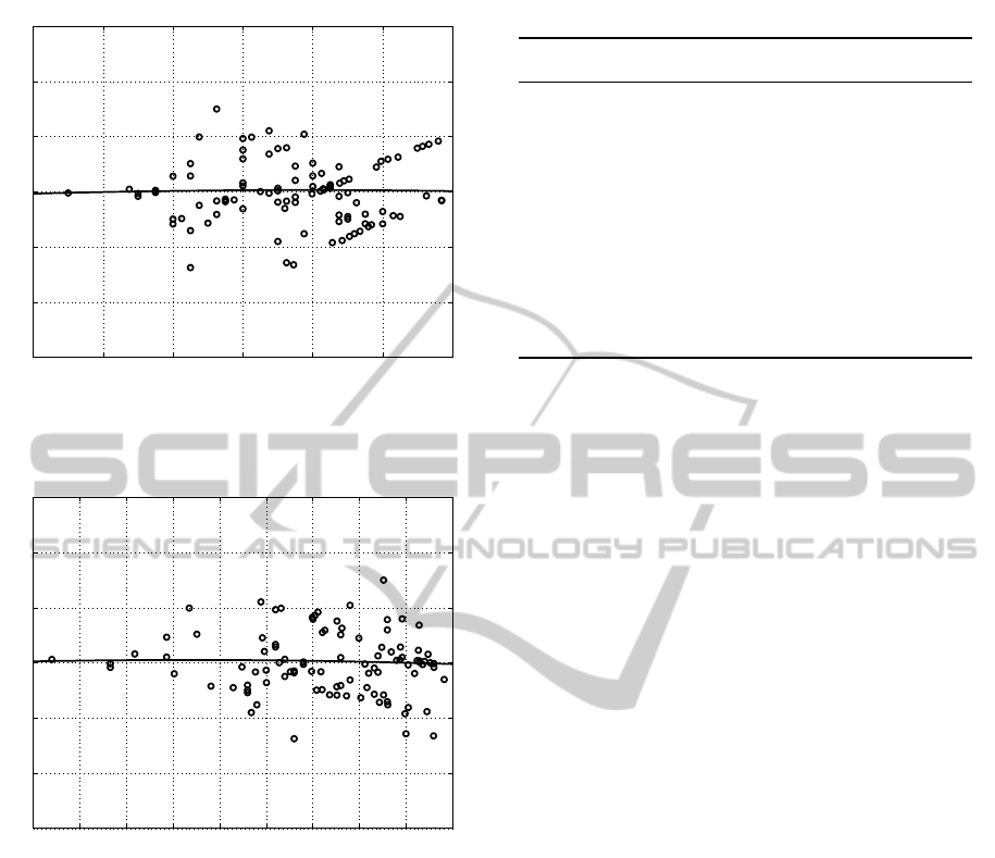
In view of this, it would be appropriate to have a

large smoothing parameter where the data are sparse,

and a smaller smoothing parameter where the data are

denser. In this situation an adaptive parameter has

been introduced. Let the ratio ν/n (where ν < n), de-

scribe the proportion of the sample which contributes

strictly positive weight to each local regression (for

example if the ratio is 0.7, it means that 70% of the

recorded data contributes to the regression). Once we

SMARTGREENS2013-2ndInternationalConferenceonSmartGridsandGreenITSystems

22 24 26 28 30 32 34

−3

−2

−1

Temperature [Celsius]

Residual

Adaptive Bandwidth: Residual vs Inside Air Temperature

Figure 4: Residual vs inside air temperature, for the user

in ﬁgures 2 and 3 using a regression in 2 variables with an

adaptive bandwidth λ for the kernel.

0 5 10 15 20 25 30 35 40 45

−3

−2

−1

Relative Humidity [%]

Residual

Adaptive Bandwidth: Residual vs Relative Humidity

Figure 5: Residual vs humidity, for the user in ﬁgures 2 and

3 using a regression in 2 variables with an adaptive band-

width λ for the kernel.

have chosen ν/n (that means we have chosen ν, as n

is ﬁxed), we select the ν nearest neighbours from the

new entry point x. Then, the smoothing parameter λ

is denoted by the distance of the most distant neigh-

bour among the ν neighbours selected. It should be

noted that the entire procedure requires the choice of

a single parameter setting. This choice generally im-

proves the previous effect, giving rise to a results as

those shown in the ﬁgures 4 and 5, where the residual

is kept more constant for both input variables.

2.2.2 The Algorithm

The proposed method can be described by the follow-

ing sequence of operations (table 1): the algorithm

is initialized by setting only one parameter (step 1).

Then, for each new entry point x (step 2), it ﬁrst com-

Table 1: Pseudocode for the proposed LRAB.

LRAB

1: Initialize: set parameters ν

2: For each entry point x:

2.1: minimise (3)

2.2: while iterations < max iterations do:

2.2.1: for each i compute (6)

2.2.2: minimise (3) replacing K

with ψ

∗ K

2.3: end while

3: end

putes an initial ﬁtting (step 2.1), then it strengthens

the initial regression by the steps 2.2.1 to 2.2.2, per-

forming the sub-procedure described in the previous

section, iteratively. If we have M new entry points x

in total, the steps from 2.1 to 2.3 are repeated M times

(one time for each new entry point).

3 EXPERIMENTS

This section describes the experimental results ob-

tained from a comparison between the proposed

method and both the Nadaraya-Watson kernel method

and the PMV method. The three kernel functions de-

scribed in section 2.1 are used to compute and com-

pare LRAB and Nadaraya-Watson methods. It should

be noted that, although PMV is not based on a learn-

ing approach, in this paper, we compare our method

with PMV since the latter is the international standard

used to predict comfort in current building design and

operation (ISO, 1994).

In particular, LRAB has been compared with

the aforementioned methods on real data from the

ASHRAE RP-884 database. This collection contains

52 studies with more than 20,000 user comfort votes

from different climate zones. However, some of these

ﬁeld studies contain only a few votes for each user.

Thus they are not well suited for testing the proposed

algorithm. This is because our approach seeks to learn

the user preferences based on their votes, and it re-

quires sufﬁciently many data records. For this reason,

only the users with more than 10 votes have been used

to compute the proposed LRAB. After removing the

studies and records as described above we were left

with 5 climate zones, 161 users and 6421 records.

LRAB has been implemented in Matlab

, using

the trust-region method to minimize the problem in

(3), with a termination tolerance of 10

−6

. The exper-

iments have been performed through leave-one-out

PersonalizedThermalComfortForecastingforSmartBuildingsviaLocallyWeightedRegressionwithAdaptiveBandwidth

validation, for each user (i.e. using a single observa-

tion from the original sample as the validation data,

and the remaining observations as the training data).

The algorithms are evaluated considering the

difference |δV| between the computed votes (by

all methods) and the actual vote (reported in the

database). As with the ﬁeld studies (Ari et al.,

2008),(Schumannet al., 2010), a prediction is deﬁned

to be accurate if |δV| < 0.7.

The computation time depends on the number of

points have to be evaluated for each prediction; for

example, we’ve found that for predictions involving

100 records they take, on average, less than 5 seconds.

In the following tables 2, 3 and 4 are reported the

comparison (in terms of percentage of success) be-

tween LRAB, Nadaraya-Watson and PMV using re-

spectively one, two and three variables.

Table 2: Comparison between LRAB, Nadaraya-Watson

and PMV using only one variable for LRAB and Nadaraya-

Watson, giving percentage accuracies.

Temperature MRT Humidity

PMV 38.47

LRAB

Tricube 64.69 64.42 57.78

Epanechnikov 64.44 64.34 55.91

Gaussian 60.06 61.11 51.90

Nadaraya-Watson

Tricube 49.48 50.19 40.11

Epanechnikov 52.07 53.38 41.89

Gaussian 51.61 52.21 35.55

Tables 2, 3 and 4 illustrate how accurately the

LRAB predicts the actual comfort vote of each user

compared with Nadaraya-Watson and PMV. With

only one variable, LRAB achieves more than 64%

accuracy (using both tricube and Epanechnikov ker-

nels), while PMV only achieves 38% accuracy.

The other considered kernel method, the Nadaraya-

Watson method with 52 − 53% accuracy also im-

proves on the PMV method, but doesn’t match the

accuracy of the proposed LRAB method. Similarly

results are shown in Tables 3 and 4 for respectively

two and three variables. In particular, the best result is

achieved with three variables where LRAB achieves

69% accuracy with both tricube and Epanechnikov

kernels.

Moreover, one can argue that kernel methods, un-

like PMV, are essentially methods that learn from the

Table 3: Comparison between LRAB, Nadaraya-Watson

and PMV using two variables for LRAB and Nadaraya-

Watson, giving percentage accuracies.

Temp. and Hum. Temp. and MRT

PMV 38.47

LRAB

Tricube 66.70 67.03

Epanechnikov 65.91 65.84

Gaussian 65.70 65.14

Nadaraya-Watson

Tricube 39.81 50.87

Epanechnikov 41.12 50.22

Gaussian 38.22 49.81

Table 4: Comparison between LRAB, Nadaraya-Watson

and PMV using three variables for LRAB and Nadaraya-

Watson, giving percentage accuracies.

Temp., Hum and MRT

PMV 38.47

LRAB

Tricube 69.27

Epanechnikov 69.22

Gaussian 65.01

Nadaraya-Watson

Tricube 45.17

Epanechnikov 43.63

Gaussian 50.19

data, and so they require a sufﬁcient amount of data

to give the best results. To test the inﬂuence of the

amount of data on the proposed LRAB, we’ve statisti-

cally investigated this effect on a subset of users from

the database (ASHRAE, RP-884). This subset in-

cludes 39 users, with at least 110 comfort votes from

each single user. We investigated the variation of the

percentage of success (according to the accuracy level

|δV| < 0.7) of the LRAB and Nadaraya-Watson using

three input variables, and the PMV, varying the num-

ber of samples used for the above methods in a range

from 10 to 110 samples. The results are shown in ﬁg-

ure 6, showing that from 50 to 110 samples, the accu-

racy of the LRAB (80% in this case) remains roughly

constant. Hence, based on this investigation, we can

SMARTGREENS2013-2ndInternationalConferenceonSmartGridsandGreenITSystems

10 20 30 40 50 60 70 80 90 100 110

0.1

0.2

0.3

0.4

0.5

0.6

0.7

0.8

0.9

Number of samples

Accuracy

Figure 6: Accuracy vs number of samples using 3 variables

for: LRAB (circle dots), Nadaraya-Watson (square dots)

and PMV (diamond dots).

conclude that the level of accuracy certainly is biased

by the amount of data used in the regression, but this

is true especially for a small amount of data, and the

results do not show much improvement after a certain

threshold. Finally, we can also see that LRAB over-

comes the Nadaraya - Watson method for almost the

entire tested range (from 20 up to 110 samples).

4 CONCLUSIONS

In the present paper, we have proposed the use of

robust locally weighted regression with an adaptive

bandwidth to predict individual thermal comfort. The

approach has been characterized and compared with

an other standard kernel method (i.e. the Nadaraya-

Watson method) and with the traditional PMV ap-

proach. The experiments were carried out using pub-

licly available datasets: they have shown that our

LRAB outperforms both Nadaraya-Watson and the

traditional PMV approaches in predicting thermal

comfort. We also investigated the inﬂuence of the

amount of the data used by LRAB on its performance,

concluding that the performance only degrades when

the predicted value is based on just a small number

of samples (less than 40 in this case). Since LRAB

can be computed quickly, and requires only a single

parameter setting that is easily obtained, then if in-

dividual comfort responses are available, this method

is feasible for use as a comfort measure in real time

control. The next step will the extension of the present

work to a similar and more challenging context: bal-

ancing the preferences of a number of different oc-

cupants sharing the same space in buildings (shared

ofﬁces)(Wilson, 2012).

This work is part of the Strategic Research Cluster

project ITOBO (supported by the Science Foundation

Ireland), for which we are acquiring occupantcomfort

reports and ﬁne grained sensor data, and construct-

ing validated physical models of the building and its

HVAC systems. The intention is then to use the com-

fort reports and sensor data as input to our LRAB

method, and then to use the output of LRAB as the in-

put to intelligent control systems which optimise the

internal comfort for the speciﬁc individual occupants.

ACKNOWLEDGEMENTS

This work is supported by Intel Labs Europe

and IRCSET through the Enterprise Partnership

Scheme, and also in part by Science Foundation Ire-

land through SFI Research Cluster ITOBO (grant

No. 07.SRC.I1170), and grant No. 08/PI/I1912.

REFERENCES

Ari, S., Wilcoxen, P., Khalifa, H., Dannenhoffer, J., and

Isik, C. (2008). A practical approach to individual

thermal comfort and energy optimization problem. In

Fuzzy Information Processing Society, 2008. NAFIPS

2008. Annual Meeting of the North American, pages 1

–6.

ASHRAE (2010). ASHRAE Standard: Thermal Environ-

mental Conditions for Human Occupancy. ASHRAE.

Atthajariyakul, S. and Leephakpreeda, T. (2005). Neural

computing thermal comfort index for HVAC systems.

Bingxin, M., Jiong, S., and Yanchao, W. (2011). Ex-

perimental design and the GA-BP prediction of hu-

man thermal comfort index. In Natural Computation

(ICNC), 2011 Seventh International Conference on,

volume 2, pages 771 –775.

Bishop, C. M. (2006). Pattern Recognition and Machine

Learning.

Busch, J. F. (1992). A tale of two populations: thermal

comfort in air-conditioned and naturally ventilated of-

ﬁces in Thailand. Energy and Buildings, 18(3-4):235

– 249.

Cleveland, W. S. (1979). Robust locally weighted regres-

sion and smoothing scatterplots. Journal of the Amer-

ican Statistical Association, 74(368):pp. 829–836.

Cleveland, W. S. and Devlin, S. J. (1988). Locally weighted

regression: An approach to regression analysis by lo-

cal ﬁtting. Journal of the American Statistical Associ-

ation, 83(403):pp. 596–610.

Daum, D., Haldi, F., and Morel, N. (2011). A personal-

ized measure of thermal comfort for building controls.

Building and Environment, 46(1):3–11.

de Dear, R. and Schiller Brager, G. (2001). The adap-

tive model of thermal comfort and energy conserva-

tion in the built environment. International Journal of

Biometeorology, 45:100–108.

PersonalizedThermalComfortForecastingforSmartBuildingsviaLocallyWeightedRegressionwithAdaptiveBandwidth

de Dear, R. J. and Brager, G. S. (2002). Thermal comfort

in naturally ventilated buildings: revisions to ashrae

standard 55. Energy and Buildings, 34(6):549 – 561.

Fanger, P. (1972). Thermal comfort: analysis and appli-

cations in environmental engineering. McGraw-Hill,

New York.

Federspiel, C. C. and Asada, H. (1992). User-adaptable

comfort control for HVAC systems. In American Con-

trol Conference, 1992, pages 2312 –2319.

Feldmeier, M. and Paradiso, J. A. (2010). Personalized hvac

control system. In In Internet of Things 2010 Confer-

ence.

Freire, R. Z., Oliveira, G. H., and Mendes, N. (2008). Pre-

dictive controllers for thermal comfort optimization

and energy savings. Energy and Buildings, 40(7):1353

– 1365.

Gagge, A. P., Fobelets, A. P., and Berglund, L. G. (1986).

A standard predictive index of human response to the

thermal environment.

Hastie, T., Tibshirani, R., and Friedman, J. H. (2003). The

Elements of Statistical Learning. Springer, corrected

edition.

Humphreys, M. and Nicol, J. (2000). Effects of measure-

ment and formulation error on thermal comfort in-

dices in the ashrae database of ﬁeld studies. ASHRAE

transactions, 106:493–502.

Humphreys, M. A. and Nicol, J. F. (2002). The valid-

ity of iso-pmv for predicting comfort votes in every-

day thermal environments. Energy and Buildings,

34(6):667 – 684.

ISO (1994). ISO 7730: Moderate Thermal Environments—

Determination of the PMV and PPD Indices and Spec-

iﬁcation of the Conditions for Thermal Comfort. ISO.

Kumar, S. and Mahdavi, A. (2001). Integrating thermal

comfort ﬁeld data analysis in a case-based building

simulation environment. Building and Environment,

36(6):711 – 720.

Olesen, B. W. (2004). International standards for the indoor

environment. Indoor Air, 14:18–26.

Schumann, A., Wilson, N., and Burillo, M. (2010). Learn-

ing user preferences to maximise occupant comfort in

ofﬁce buildings. In Proceedings of the 23rd interna-

tional conference on Industrial engineering and other

applications of applied intelligent systems - Volume

Part I, IEA/AIE’10, pages 681–690, Berlin, Heidel-

berg. Springer-Verlag.

Sherman, M. (1985). A simpliﬁed model of thermal com-

fort. Energy and Buildings, 8(1):37 – 50.

Shukor, S. A. A., Kohlhof, K., and Jamal, Z. A. Z.

(2007). Development of a pmv-based thermal com-

fort modelling. In Proceedings of the 18th IASTED

International Conference: modelling and simulation,

MOAS’07, pages 670–675, Anaheim, CA, USA.

ACTA Press.

Wilson, N. (2012). On balancing occupants’ comfort in

shared spaces. In Proc. 6th Multidisciplinary Work-

shop on Advances in Preference Handling (MPREF-

12).

Yang, K. and Su, C. (1997). An approach to building energy

savings using the PMV index. Building and Environ-

ment, 32(1):25 – 30.

Yang, W. and Zhang, G. (2008). Thermal comfort in nat-

urally ventilated and air-conditioned buildings in hu-

mid subtropical climate zone in china. International

Journal of Biometeorology, 52:385–398.

SMARTGREENS2013-2ndInternationalConferenceonSmartGridsandGreenITSystems