
Submeter based Training of Multi-class Support Vector Machines for
Appliance Recognition in Home Electricity Consumption Data
Marco Mittelsdorf
1
, Andreas H
¨
uwel
2
, Thole Klingenberg
2
and Michael Sonnenschein
2
1
Department of Computing Science, University of Oldenburg, Oldenburg, Germany
2
OFFIS - Institute for Information Technology, Oldenburg, Germany
Keywords:
Appliance Recognition, Smart Metering, Submetering, Energy Monitoring, Multi-class Support Vector
Machines.
Abstract:
In this paper we employ smart meter and support vector machines (SVM) for the problem of recognizing
household appliances’ load patterns in measured load time series, which is an important step for various
applications in energy consulting, process recognition or health care applications. We present an automated
data collection and preprocessing approach that intrinsically avoids many privacy (and security) issues by
keeping the whole process local to the household. In the experimental part we investigate multi-class SVMs in
the problem domain of automatically recognizing appliances in load profiles of smart meters. For the learning
phase, we use low intrusive submeters to automatically and locally generate household specific test data for the
supervised training and validation of the SVMs. We analyze classifiers w.r.t. various training sets and feature
spaces. Comparing data from household simulator and real household data, we find that excellent recognition
rates can be achieved even with low resolution data and rather unsophisticated feature space.
1 INTRODUCTION
The energy transition towards Smart Grid forces en-
ergy consumers to adapt to the capabilities of energy
producers. This also effects private households. From
a more or less passive role that can be characterized
by standard load profiles they need to become more
aware of the effects of their own energy consumption.
Thus a major goal of all customer information,
feedback or consulting systems for electricity con-
sumption is to motivate and deepen the residents un-
derstanding of energy consumption, and to possi-
bly trigger investments in energy efficiency or even
start changes in behaviour towards a smarter con-
sumption. As suggested by Raabe, Sonnenschein,
Beenken, H
¨
uwel and Meinecke (2012) an energy con-
sulting system for private households should give
feedback and hints on how to reduce the overall en-
ergy consumption on the level of appliance usage.
Smart metering is widely discussed for data acqui-
sition in such scenarios. While the global aim is to
give insight into power consumption of individual or
grouped household appliances, real world scenarios
often have the restriction of keeping data acquisition
and processing privacy-compliant. This often means
that only those aggregated meter data are to leave the
household, that are strictly necessary in respect of in-
voicing. Any further data, for example needed for
the consulting system, must not be transferred some-
where else. The locally gathered total load of the
household must be disaggregated into the individual
consumption values of each appliance, which is in the
fields of Non-Intrusive Appliance Load Monitoring
(NIALM). So, in this paper one focus lies on locally
labelling the smart meter data, needed for the super-
vised training phase of our appliance recognition. An-
other focus is to perform an analysis of different sce-
narios, how feature space and sampling rate affects
event detection and classication.
The rest of this paper is structured as follows. In
section 2 we give a short introduction to related ap-
proaches in NIALM and in appliance recognition us-
ing support vector machines (SVM). In section 3 we
present the methodological background that our ap-
pliance recognition approach builds on. In section 4
we present our appliance recognition approach and in
section 5 we describe our evaluation scenarios and the
results of our classifiers. In section 6 we summarize
our approach and the results.
151
Mittelsdorf M., Hüwel A., Klingenberg T. and Sonnenschein M..
Submeter based Training of Multi-class Support Vector Machines for Appliance Recognition in Home Electricity Consumption Data.
DOI: 10.5220/0004380001510158
In Proceedings of the 2nd International Conference on Smart Grids and Green IT Systems (SMARTGREENS-2013), pages 151-158
ISBN: 978-989-8565-55-6
Copyright
c
2013 SCITEPRESS (Science and Technology Publications, Lda.)

2 RELATED WORK
Zeifman, Akers and Roth (2011) give an exhaustive
overview over various NIALM approaches that were
untertaken between the introduction of the concept by
Hart (1992) and today. In this work we focus on su-
pervised learning approaches in order to recognize ap-
pliance switching events. For that we need a training
phase to train classifiers using labelled data. The qual-
ity of such approaches depends strongly on reliable
training sets (regarding the labels), the choice of fea-
ture space and time resolution of the underlying data.
Following Hart (1992) the time resolution of con-
sidered load series must at least be in the range of
individual usages of appliances for the purpose of ap-
pliance classification. This is mostly a few seconds
to subseconds. Some systems even sample at sev-
eral kilohertz, like the one of Leeb, Shaw and Kirt-
ley (1995), the one of Matthews, Soibelman, Berges
and Goldman (2008) or the one of Zeifman and Roth.
Their approaches need sophisticated sensory but com-
pared to 1 Hz solutions they enable a new stack of
means to the classification problem, which is not fo-
cused in this paper.
When using NIALM one major question is how
to create the training data and the classifiers. Pi-
hala (1998) gathered his ex ante data of few types of
larger appliances over several years in separate field
studies, thus once productive the classifiers cannot be
further adopted to a specific household. The feedback
system of Mattern, Staake and Weiss (2010) allows
the consumer himself to manually perform point-wise
measurements of a single household appliance, like
for instance the power consumption of the computer
getting switched on. Lacking an automated approach,
the training phase still must be done manually by the
consumer himself and this is easily getting tedious
and error prone.
When looking beyond the ”few large” standard
household appliances the system must be able to up-
date the training data and retrain the classifiers. This
can either be done by data exchange to the outside of
the household or to locally sample and retrain. While
Weiss, Staake, Mattern and Fleisch (2012) suggest a
system that offensively goes public, real world field
scenarios often must be compliant to a more restrict-
ing privacy policy, where only those aggregated data
may be exchanged to the utility, that are needed for
invoicing.
In the context of appliance recognition support
vector machines (SVM) can be used to conduct a
classification of whether a given switching event was
caused by a certain household appliance or not. Based
upon training data the SVM constructs a hyperplane,
which separates the items of two classes and allows
to classify new observations by simply determining
on which side of the hyperplane it lies.
In previous NIALM systems SVMs have mostly
been applied to data that was measured using sen-
sors with high sample rates of at least several kHz.
To our knowledge Onoda, Murata and Ratsch (2002)
were the first to employ SVMs for the task of es-
timating the state of electric household appliances
based on harmonic information. Patel, Robertson,
Kientz, Reynolds and Abowd (2007) computed the
Fast Fourier Transformation of transient noise signals
and used it as a feature. They did also employ SVMs
for classification. Lin (2011) stressed that the NIALM
problem is in fact a multiple-class decision prob-
lem. Very recently Jiang, Luo, and Li (2012) applied
multi-class support vector machines (MC-SVMs) to
the NIALM problem.
Our approach aims at typical smart meters, which
usually have to make use of low cost hardware in or-
der to enable large scale rollouts. This results in rather
low sample rates in the range of 15 minutes to one sec-
ond. So instead of harmonic features we rely on the
steady-states and transient variations of the electric
load that can be measured with such low frequency
sensors.
Kramer et al. (2012) demonstrated that appli-
ance recognition based on such low frequency fea-
tures can be solved with ensembles of MC-SVMs
and K-Nearest Neighbor (KNN) classifiers. They
achieved recognition rates of around 95 % with the
ensemble classifier on a test set consisting of 15 ap-
pliances. Furthermore they show that the ensemble
classifier outperforms a MC-SVM based on a RBF
kernel which yielded recognition rates from 90.5 % to
94.3 % on the same dataset.
3 DATA ACQUISITION
Our system is designed to stay compliant to a strict
privacy policy, which would not allow any exchange
of non aggregated power consumption or training
data. To gather the needed training data under such
determining factors, we adopt an appliance recogni-
tion approach similar to the NIALM approach by us-
ing low intrusive submeters during the needed train-
ing phase. Avoiding error prone manual labelling,
they automatically create our training data keeping
the whole process local to the household.
Before we introduce our appliance recognition ap-
proach we introduce the data our experimental study
is based on. We employ two kinds of data sets. First
is data that contains measurements of everyday appli-
SMARTGREENS2013-2ndInternationalConferenceonSmartGridsandGreenITSystems
152

ances which are turned on or off. We consider this our
validation data. We use it to evaluate whether our ap-
pliance recognition algorithm performs well on real-
world data. Second is data that was generated by our
simulation approach. We use this data to implement
and test our appliance recognition algorithm.
3.1 Real-world Data
Submetering is one possible approach to create train-
ing sets on a per household basis. As the name sug-
gests each appliance is connected to an additional
power meter, which enables us to automatically de-
cide whether the appliance is currently switched on
or off. We implemented an algorithm which executes
the following steps automatically:
1. detect switching events within the data of subme-
ters and generate labels according to the appliance
connected to the respective submeter
2. detect switching events within the smart meter
data
3. match submeter events and smart meter events by
timestamp
4. assign labels of submeter events to matching
smart meter events
For details regarding our implementation or the per-
formance of our matching algorithm please refer to
(Klingenberg, 2010). The real-world data we use in
this paper originated from such a submetering setup.
During four weeks we employed the approach for
monitoring a small group of six kitchen appliances.
The smart meter we used has a resolution of approx-
imately 17 Hz and a basic accuracy of 0.5% of full
scale (300 V, 15 A).
3.2 Simulation of Household Appliances
In order to evaluate the results of our appliance recog-
nition approach under various circumstances we em-
ploy a simulation approach. Therefore we imple-
mented a household simulator which generates the
total load profile of a model household as well as a
load profile of every single simulated appliance. This
is the same data which we acquire by employing the
abovementioned submetering approach. In order to
further improve the comparability of both approaches
the simulator does also generate data at a resolution
of 17 Hz.
The easiest way to create a simulation model of
an appliance, that reproduces steady state transitions
as well as the transient behaviour during switching
events realistically, is to record load patterns during
appliance operation. At simulation time the appliance
model steps through one, e.g. randomly chosen, pat-
tern value by value.
As was stated by Hart (1992), Pihala (1998),
Baranski (2006) and others the electric load is highly
dependent on the fluctuating voltage signal. Electric
admittances though are not influenced by the voltage
signal in theory. Admittance values are therefore a
better representation for our appliance patterns than
active and reactive power values. We do therefore use
recorded voltage signals U
a,t
and current signals I
a,t
of an appliance a to compute the admittance
Y
a,t
=
I
a,t
U
a,t
(1)
for each time step t of the signal and use it to compute
the values of conductance G
a,t
and susceptance B
a,t
by applying the following relation :
Y
i
= G
a,t
+ j · B
a,t
(2)
= Y
a,t
· (cosϕ − j · sin ϕ) (3)
which yields the calculation rules
G
a,t
= Y
a,t
· cosϕ (4)
B
a,t
= −Y
a,t
· sinϕ (5)
where ϕ = ϕ
u
− ϕ
i
denotes the phase angle between
current and voltage signal. This way we prepared a
pattern comprised of time series G
a
and B
a
for each
appliance we want to include into our simulator.
For simulation purposes we employ a simplified
electric single-phased model of households. We basi-
cally assume that all appliances are plugged together
in a parallel connection. This enables us to compute
the total admittance of the household:
Y
tot
=
N
∑
i=1
Y
i
(6)
At simulation time a predefined operation sched-
ule specifies when appliances are switched on or off.
The simulator does also generate a fluctuating voltage
signal U
0
which we use to calculate the total active
power P and reactive power Q of the household and
of each appliance according to the following formu-
las:
I = U ·Y (7)
S = U · I
∗
(8)
P = Re(S) (9)
Q = Im(S) (10)
4 OUR APPLIANCE
RECOGNITION APPROACH
Our approach is divided into the following three main
steps – here presented for the virtual household, for
the real household we use smart meter and submeter.
SubmeterbasedTrainingofMulti-classSupportVectorMachinesforApplianceRecognitioninHomeElectricity
ConsumptionData
153

1. Training of classifiers: We use the household sim-
ulator to generate labelled training data for a given
set of appliances and train a MC-SVM.
2. Scenario classification: We use the household
simulator to generate a new total load profile,
consisting of the same set of appliances and use
the MC-SVM to classify the detectable switching
events.
3. Scenario evaluation: We compare the results of
the classification process to the load profiles of
the appliances and generate a summarizing statis-
tic about matches and mismatches.
One main component of steps 1 and 2 is our event
detection and feature extraction algorithm. Therefore
we will start with a description of this algorithm be-
fore we describe the three main steps in the following
sections.
4.1 Event Detection & Feature
Extraction
Our event detection algorithm is based on the active
power signal and consists of the following six steps
and an optional seventh step. The first step is a pre-
processing operation according to the suggestion of
(Hart, 1992) to only use normalized power values for
appliance recognition. We therefore eliminate the in-
fluence of the fluctuating power signal by applying
P
normalized
= U
2
ref
· G (11)
Where U
ref
denominates the nominal value of the sup-
ply voltage and G is the electric conductance.
In the second step we compute the series of differ-
ences of this normalized power time series:
∆P
t
= P
t
− P
t−1
(12)
According to (Baranski, 2006) this representation is
well suited for the detection of switching events be-
cause they do appear as peaks whereas steady-state
segments of the load profile appear as values around
zero.
In the third step we apply a global filter to the se-
ries of differences in order to remove most of the noise
events from the signal. This global threshold is to be
carefully chosen because if it is too high it suppresses
events of some appliances. If it is chosen too low a
significantly higher amount of noise events has to be
handled during recognition phase.
In the fourth step continuous sections of positive
or negative values within the series of differences
are combined. This enables us to combine staircase-
shaped event sequences to one single event. We found
that most staircase-shaped events have a duration of
Table 1: Overview of the features we use for classification.
Feature Description
∆P Change in active power
∆Q Change in reactive power
∆Z Change in impedance
∆R Change in resistance
∆X Change in reactance
∆Y Change in admittance
∆G Change in conductance
∆B Change in susceptance
P
Surge
Maximum active power of the surge
t
Surge
Duration of the surge
less than one second. The maximal duration of a sec-
tion is therefore limited to one second. It follows that
events of different appliances need to be at least one
second away from each other.
In the fifth step all events of a section are added up.
We use the sum of the switching powers to represent
the total power of the combined switching event.
The sixth step is only necessary for extracting ac-
curate training data and is skipped during the classifi-
cation of a scenario load profile. In this step an appli-
ance specific filter is applied to separate noise events
from events that represent a relevant state change.
Noise events may occur during appliance operation.
They often have a lower power draw than on and
off events but they exceed the global filter threshold.
Switching on power surges are treated as two events.
One indicates the rising edge and the other one the
falling edge of the surge. With an optional seventh
step a surge event can be detected and combined to a
single event.
Other electric features such as reactive power,
admittance or resistance are extracted based upon
the sections which where identified in step four and
maybe further combined in step seven. The change of
these features is computed by subtracting the value at
the begin of a section from the value at the end of the
section. Table 1 gives an overview of the features we
use for classification.
4.2 Training of Classifiers
Supervised machine learning algorithms like SVM
need labelled training data. In order to generate la-
belled data of a given appliance we use submeters or
our simulator to get load profiles containing switch-
ing events of only this appliance. Next we apply
our event detection algorithm. The events of each
appliance are divided into on and off events and la-
belled respectively. Noise events which do not repre-
sent state changes of appliances are also divided into
events with ascending power change and events with
SMARTGREENS2013-2ndInternationalConferenceonSmartGridsandGreenITSystems
154

descending power change. In total 2n + 2 (2 noise
classes and 2n classes for all appliances) distinguish-
able labels are generated where n is the number of
appliances considered.
4.3 Scenario Classification
First step of the classification is to run the event detec-
tion and feature extraction algorithm on the load pro-
file to gain appropriate input data for the MC-SVM.
In the second step every event is classified.
4.4 Scenario Evaluation
During this phase we evaluate how well the classi-
fier performed during the aforementioned classifica-
tion phase. To find the true class of an event we use
the appliance load profiles which are also provided
by the household simulator. The event detection and
feature extraction algorithm is used to determine the
switching events within these load profiles. Next we
compare these events with those that were classified
earlier. If timestamp and label are equal then the clas-
sification was correct. If the timestamp matches but
the label does not then a misclassification occurred.
5 EXPERIMENTAL STUDIES
In the first part of this section we introduce three sce-
narios to test and to evaluate our system on. In the
second part we present the results of each scenario.
A full description of the scenarios and results can be
found in (Mittelsdorf, 2012).
5.1 Scenarios
Scenario 1 - Feature Space. Here we analyze the
influence of the feature selection on the appliance
recognition rates. Out of the available 27 appliances
of the household simulator we chose a subset of 18
appliances for the base scenario (1a). Two additional
appliances are considered in two variants of the base
scenario: a fridge (1b) and a washing machine (1c).
The seven remaining appliances are either not repre-
sentative because we could not capture enough data or
the event detection does not work reliably for them.
The power draw of a stereo system for instance
heavily depends on the current volume level and the
song just played. (Baranski, 2006) counts the stereo
system to continuously varying electric consumers
which are much more demanding than simple steady
state on-off-appliances with constant power draws.
Another appliance which we do not consider is for
example the 20 W desk lamp. Since a global 40 W
filter led to the best results for the majority of appli-
ances, switching events of smaller consumers are fil-
tered out.
To create scenario 1a we simulated a load pro-
file with a duration of 24 hours. All appliances were
scheduled to switch on and off several times and over-
lap in their operating time. Altogether 1230 events
were detected. Figure 1 shows that some of the ap-
pliances have a similar power draw. We presume that
by using only the active power as feature misclassifi-
cations will occur. Our assumption is therefore that
classification rates will improve by adding more fea-
tures.
Scenario 2 - Sampling Rate. In order to investigate
the influence of the sampling rate on appliance recog-
nition we use the same scenario with a 17 Hz and a
1 Hz sampling rate. The latter one is created by down-
sampling the load profile of the 17 Hz scenario. The
appliance set of this scenario consists of an incandes-
cent lamp, a water kettle, a vacuum cleaner and a TV.
The lamp has a low and the water kettle a high power
draw. The TV and the vacuum cleaner show a power
surge in their load profiles whereas the other two ap-
pliances do not. The set therefore covers appliances
with different characteristics.
Scenario 3 - Real Data. In order to investigate the
performance of our system applied to real world data
we compare the classification results achieved on the
real world data mentioned in section 3.1 to the results
of simulated load profiles. The real world data we
use was recorded by (Klingenberg, 2010) and consists
five appliances: dishwasher, fridge, coffee maker,
boiler and water kettle.
5.2 Results
Out of the confusion matrix various classification pa-
rameters can be calculated. We use the hit rate, false
alarm rate, precision and ROC-Score. We extended
the classical confusion matrix for two class problems
to our multi-class classification approach. Figure 2
shows this for the switch-off class of the fridge. While
the true positive rate TP is still a single value false
negative FN, false positive FP and true negative rates
TN now represent the summarized values of the ac-
cordingly row (FN), column (FP) or main diagonal
(TN).
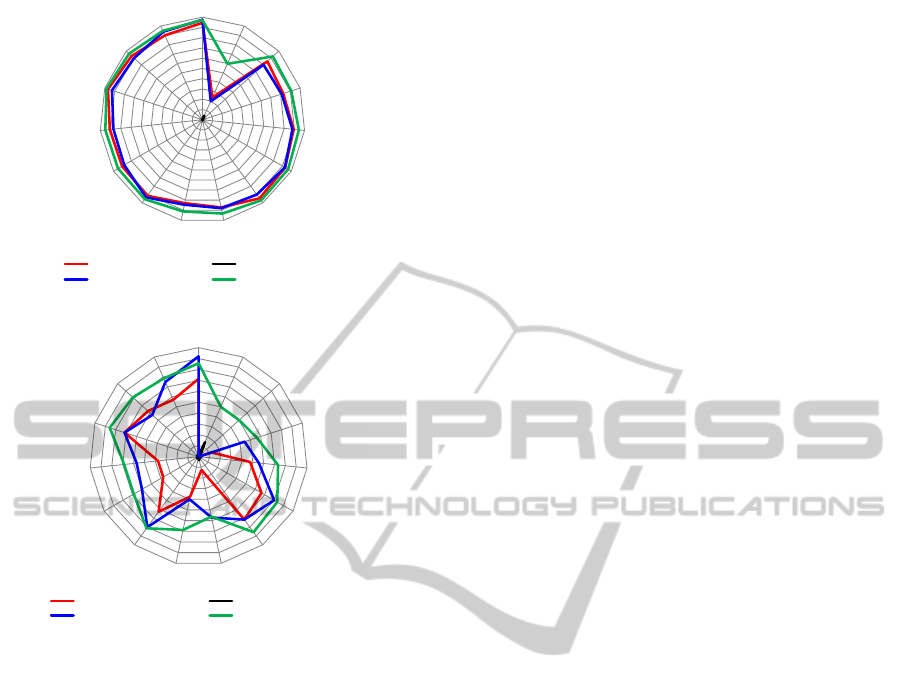
Scenario 1 - Feature Space. The results of scenario
1a are presented in Figure 3. It shows the four classifi-
cation parameters for different features. The upper di-
SubmeterbasedTrainingofMulti-classSupportVectorMachinesforApplianceRecognitioninHomeElectricity
ConsumptionData
155

-2.750 -2.500 -2.250 -2.000 -1.750 -1.500 -1.250 -1.000 -750 -500 -250 0 250 500 750 1.000 1.250 1.500 1.750 2.000 2.250 2.500 2.750 3.000
P in W
Buegeleisen_01
Energiesparlampe_01
Gluehbirne_01
Fernseher_01
Haartrockner_01
Haartrockner_02
Haartrockner_03
Kaffeemaschine_01
Kafcaf emaschine_02
Mikrowelle_01
Staubsauger_01
Toaster_01
Toaster_02
Wasserkocher_01
Wasserkocher_02
Wasserkocher_03
Wasserkocher_04
Wasserkocher_05
Electric kettle 05
Electric kettle 04
Electric kettle 03
Electric kettle 02
Electric kettle 01
Toaster 01
Toaster 02
Vacuum cleaner 01
Microwave 01
Hair dryer 03
Coffee machine 01
Coffee machine 02
Hair dryer 02
Hair dryer 01
TV 01
Incandescent lamp 01
Flat iron 01
Energy saving lamp 01
Figure 1: Distribution of switching power from the appliances of scenario 1. Areas of similar switching power of two or more
appliances are highlighted red.
agram shows mean values whereas the lower diagram
shows the worst achieved values for a single class.
The best results were achieved by using the features
(∆P) and (∆P, ∆Z). The mean hit rate for (∆P) was
96.25 % and for (∆P, ∆Z) was 96.2 %. The worst hit
rate for (∆P) was 70 % as the lower diagram shows,
which means that at least for one class only 70 % of
the switching events were classified correctly. Most
of the feature combinations used in scenario 1 have
satisfying mean results as the upper diagram in Fig-
ure 3 shows, but for some combinations worse results
were achieved for a single class. The minimal hit rate
with the features (∆P, ∆Q, ∆Y ) was 0 % which means
switching events of one class haven’t been classified
correctly at all. Therefore this combination is not
suitable for our appliance recognition system. Other
unsuitable features are (∆Q), (∆B) and (∆X) which
have a mean hit rate of less than 25 %.
In scenario 1b we added a fridge and in scenario
1c we added a washing machine as additional appli-
ances to the base scenario. The mean hit rate for sce-
nario 1b was 93 % and for scenario 1c only 85.94 %.
The worse results of scenario 1c can be explained by
the high number of switching events that occur during
washing machine operation and their different switch-
ing powers. The majority of the washing machine
switching events have a switching power in the range
of 40 W to 400 W and -40 W to -400 W. Eight out of
=== Detailed Accuracy By Class ===
Total Number of Instances: 1150
Correctly Classified Instances: 996 86,609 %
Incorrectly Classified Instances: 154 13,391 %
HIT FAR PRE ROC
83,333 0 1 91,667 Geschirrspueler_Real_off
1 0 1 1 Geschirrspueler_Real_on
98,913 8,122 53,216 95,396 Kaffeemaschine_Real_off
1 0 1 1 Kaffeemaschine_Real_on
78,168 3,409 95,024 87,379 Kuehlschrank_Real_off
95,973 1,114 97,279 97,429 Kuehlschrank_Real_on
1 0,102 93,750 99,949 Wasserboiler_Real_off
93,333 0 1 96,667 Wasserboiler_Real_on
94,595 3,223 52,239 95,686 Wasserkocher_Real_off
74,074 1,215 62,500 86,430 Wasserkocher_Real_on
47,059 0 1 73,529 noise_off
1 0 1 1 noise_on
47,059 0,000 52,239 73,529 minimum
100,000 8,122 100,000 100,000 maximum
88,787 1,432 87,834 93,678 mean
86,609 2,593 90,834 92,008 weighted average
Legend: HIT = Hit Rate, FAR = False Alarm Rate, PRE = Precision,ROC = ROC-Score
=== Confusion Matrix ===
a1 b1 c1 d1 e1 f1 g1 h1 i1 j1 k1 l1 <== classified as
5 . . . 1 . . . . . . . a1 = Dishwasher_Real_off
. 4 . . . . . . . . . . b1 = Dishwasher_Real_on
. . 91 . 1 . . . . . . . c1 = Coffee_machine_Real_off
. . . 88 . . . . . . . . d1 = Coffee_machine_Real_on
. . 80 . 401 . . . 32 . . . e1 = Fridge_Real_off
. . . . . 286 . . . 12 . . f1 = Fridge_Real_on
. . . . . . 15 . . . . . g1 = Boiler_Real_off
. . . . . 1 . 14 . . . . h1 = Boiler_Real_on
. . . . 1 . 1 . 35 . . . i1 = Electric_kettle_Real_off
. . . . . 7 . . . 20 . . j1 = Electric_kettle_Real_on
. . . . 18 . . . . . 16 . k1 = Noise_off
. . . . . . . . . . . 21 l1 = Noise_on
FN
FP
TN
TP
Figure 2: Confusion matrix of multi-class classification.
the 18 appliances show also switching powers in this
range, so it is more likely that events of those ap-
pliances are classified as washing machine and vice
versa washing machine events are classified as events
of those appliances.
Scenario 2 - Sampling Rate. Let us look at the ac-
curacy of the event detection at both sampling rates.
In case of the 17 Hz sampling rate the event detection
works precisely and detects all events of the four ap-
pliances we use in this scenario. Applied to the 1 Hz
data, the event detection misses 11 out of 151 events.
0
20
40
60
80
100
P
G
Q
B
R
Y
Z
X
PQ
GB
PZ
PY
PR
PX
PQZ
PQY
PQR
PYR
PZR
mean hit rate
mean false alarm rate
mean precision
mean ROC-Score
0
20
40
60
80
100
P
G
Q
B
R
Y
Z
X
PQ
GB
PZ
PY
PR
PX
PQZ
PQY
PQR
PYR
PZR
minimal hit rate
maximal false alarm rate
minimal precision
minimal ROC-Score
Figure 3: Classification results for different features of sce-
nario 1a in percentage. Mean results of all classes on the
top and worst results of a single class on the bottom.
SMARTGREENS2013-2ndInternationalConferenceonSmartGridsandGreenITSystems
156
0
10
20
30
40
50
60
70
80
90
100
P
Q
Z
R
Y
PQ
PZ
ZR
ZQ
PZY
PZQ
PQZRXYGB
PPs
PPsTsQZRXYGB
PPsQ
mean hit rate
mean false alarm rate
mean precision
mean ROC-Score
0
10
20
30
40
50
60
70
80
90
100
P
Q
Z
R
Y
PQ
PZ
ZR
ZQ
PZY
PZQ
PQZRXYG
B
PPs
PPsTsQZ
RXYGB
PPsQ
minimal hit rate
maximal false alarm rate
minimal precision
minimal ROC-Score
Figure 4: Classification results for different features of sce-
nario 3. Mean results of all classes on the top and worst
results of a single class on the bottom.
This leads to an accuracy of 92.72 %. If the noise
events are also considered then only 87 % of the 17 Hz
events were detected in the 1 Hz data.
The quality of the classification results also de-
pends heavily on the sampling rate. On the 17 Hz data
we could achieve an average hit rate of 90.62 %. The
hit rate achieved on the 1 Hz data was significantly
worse and amounted to 74.64 %.
The lower accuracy of both event detection and
classification combines to dramatically lower accu-
racy of the whole appliance recognition system.
Scenario 3 - Real World Data. The best result was
achieved with the features (∆P, P
Surge
) with a mean hit
rate of 96.8 %. Also the features (∆P) and (∆P, ∆Z)
led to good classification results as Figure 4 shows.
The evaluation of the real world scenario shows simi-
lar results as for the simulated data. From this we con-
clude that our simulator is suitable to generate data
close enough to reality.
6 DISCUSSION
In this work we demonstrated how an appliance
recognition system can be set up by the use of subme-
tering data. We presented the concept of our house-
hold simulator which allows us to design and generate
load profiles of a model household and of single ap-
pliances for testing purposes. We also presented our
appliance recognition algorithm which was tested on
such simulated data and on a real world dataset.
We investigated which choice of features leads to
the best results in appliance recognition using MC-
SVMs. Therefore we performed a feature study on
simulated and on a real world scenarios. In both cases
most scenarios have shown satisfying recognition re-
sults, if the change of active power ∆P is among the
considered features. Also the feature combinations
(∆P) or (∆P, ∆Z) which perform best on simulated
data did perform very well on the real world data.
These results indicate that our simulator is a reason-
able model of real households. A more systematic
approach to validate our household simulator might
be to recreate a real world scenario using simulation
models of the exact same appliances that were used in
reality. The two resulting load profiles could be com-
pared by calculating the residual sum of least squares,
which should ideally have the value zero.
Most appliance recognition systems rely on data
with a resolution of several kHz or on data with a res-
olution of 1 Hz. We investigated how the recognition
rates behave if slightly higher resolutions than 1 Hz,
such as 17 Hz, are used. Based on the findings from
our scenario appliance recognition systems at 17 Hz
do significantly outperform systems at 1 Hz. The rea-
son is that the 1 Hz system drops more events dur-
ing event detection and in addition it recognizes only
about 75 % correctly during event classification.
On the real world data we were able to achieve
a recognition rate of 96.8 % with the feature combi-
nation (∆P, P
Surge
). (Kramer et al., 2012) used the
same sensor as we did and achieved recognition rates
of up to 95 % with ensemble classifiers created from
SVM and KNN classifiers. They found recognition
rates ranging from 90.5 % to 94.3 % using a MC-
SVM based on an RBF kernel. On the first glance
our algortihm performs better, but it should be men-
tioned that our real world data consists of five in-
dividual appliances whereas the data investigated by
(Kramer et al., 2012) consists of 15 individual appli-
ances. So the complexity of their classification prob-
lem is higher. On the other hand the data investigated
by (Kramer et al., 2012) consists of hand-picked,
manually labelled patterns and is balanced whereas
our dataset was automatically detected whithin data
SubmeterbasedTrainingofMulti-classSupportVectorMachinesforApplianceRecognitioninHomeElectricity
ConsumptionData
157

from everyday life and automatically annotated us-
ing the additional data of submeters. Since we aim
for a fully automated approach we additionally have
to automate the decision whether an event originated
from the state change of an appliance or from noise
in the power signal. We incorporated this decision
into the classification problem by adding additional
classes for noise events.
We addressed privacy indirectly by designing our
system in a way that allows us to train classifiers on
a per household basis. This means that all personal
data is processed in-house and never uploaded or pro-
cessed anywhere else.
One drawback of our system is, that all classifiers
have to be retrained if a new appliance is added to the
household. In such a case the data of most appliances
can be reused, but during a short setup phase patterns
of the new appliance must be gathered. So at least
one submeter should permanently be available in the
household whereas most other submeters can be re-
moved after the initial setup.
ACKNOWLEDGEMENTS
This work has been supported by funds of the
Federal Ministry of Economy and Technology in
the E-Energy project eTelligence, project number
01MR08007A.
REFERENCES
Baranski, M. (2006). Energie-Monitoring im privaten
Haushalt. PhD thesis, University of Paderborn.
Hart, G. (1992). Nonintrusive appliance load monitoring.
Proceedings of the IEEE, 80(12):1870 –1891.
Jiang, L., Luo, S., and Li, J. (2012). An Approach of House-
hold Power Appliance Monitoring Based on Machine
Learning. 2012 Fifth International Conference on
Intelligent Computation Technology and Automation,
pages 577–580.
Klingenberg, T. (2010). Smart Submetering - Effizien-
ter Einsatz von Submetern zur Aktivit
¨
atsbestimmung
in Privathaushalten mit Hilfe adaptiver Lernverfahren.
Master’s thesis, University of Oldenburg.
Kramer, O., Wilken, O., Beenken, P., Hein, A., H
¨
uwel, A.,
Klingenberg, T., Meinecke, C., Raabe, T., and Son-
nenschein, M. (2012). On ensemble classifiers for
nonintrusive appliance load monitoring. 7th Inter-
national Conference on Hybrid Artificial Intelligence
Systems (HAIS), pages 322–331.
Leeb, S. B., Shaw, S. R., and Kirtley, J. L. (1995). Transient
Event Detection in Spectral Envelope Estimates. IEEE
Transactions on Power Delivery, 10(3):1200–1210.
Lin, Y.-h. and Tsai, M.-S. (2011). Applications of hierarchi-
cal support vector machines for identifying load oper-
ation in nonintrusive load monitoring systems. 2011
9th World Congress on Intelligent Control and Au-
tomation, pages 688–693.
Mattern, F., Staake, T., and Weiss, M. (2010). ICT for
green: how computers can help us to conserve en-
ergy. International Conference on Energy-Efficient
Computing and Networking.
Matthews, H. S., Soibelman, L., Berges, M., and Goldman,
E. (2008). Automatically disaggregating the total elec-
trical load in residential buildings: a profile of the re-
quired solution. In International Workshop on Intelli-
gent Computing in Engineering, page 381389.
Mittelsdorf, M. (2012). Evaluierung des Einflusses
von Merkmalsauswahl und Abtastrate auf die
Ger
¨
ateerkennung mit Support-Vektor-Maschinen.
Master’s thesis, University of Oldenburg.
Onoda, T., Murata, H., and Ratsch, G. (2002). Experimen-
tal analysis of support vector machines with different
kernels based on non-intrusive monitoring data. Neu-
ral Networks, 2002., pages 2186–2191.
Patel, S., Robertson, T., Kientz, J., Reynolds, M., and
Abowd, G. (2007). At the flick of a switch: De-
tecting and classifying unique electrical events on the
residential power line (nominated for the best paper
award). In Krumm, J., Abowd, G., Seneviratne, A.,
and Strang, T., editors, UbiComp 2007: Ubiquitous
Computing, volume 4717 of Lecture Notes in Com-
puter Science, pages 271–288. Springer Berlin Hei-
delberg.
Pihala, H. (1998). Non-intrusive appliance load monitor-
ing system based on a modern kWh-meter. Technical
Research Centre of Finland.
Raabe, T., Sonnenschein, M., Beenken, P., H
¨
uwel, A., and
Meinecke, C. (2012). Energieberatung in haushal-
ten auf basis des smartmetering.
¨
Okologisches
Wirtschaften, 1:46–50.
Weiss, M., Staake, T., Mattern, F., and Fleisch, E. (2012).
Powerpedia: changing energy usage with the help of
a community-based smartphone application. Personal
and Ubiquitous Computing, 16(6):655–664.
Zeifman, M., Akers, C., and Roth, K. (2011). Nonintrusive
appliance load monitoring (nialm) for energy control
in residential buildings. International Conference on
Energy Efficiency in Domestic Appliances and Light-
ing (EEDAL), Copenhagen.
Zeifman, M. and Roth, K. (2011). Nonintrusive appliance
load monitoring: Review and outlook. IEEE Transac-
tions on Consumer Electronics, 57(1):76–84.
SMARTGREENS2013-2ndInternationalConferenceonSmartGridsandGreenITSystems
158
