
Mining Japanese Collocation by Statistical Indicators
Takumi Sonoda and Takao Miura
Dept. of Elect. and Elect. Engineering, HOSEI University, Kajinocho 3-7-2, Koganei, Tokyo, Japan
Keywords:
Collocation, Co-occurrences, Feature Selection, Natural Language Processing.
Abstract:
In this investigation, we discuss a computational approach to extract collocation based on both data mining
and statistical techniques. We extend n-grams consisting of independent words and that we take frequencies
on them after filtering on colligation. Then we apply statistical filters for the candidates, and compare these
feature selection methods in statistical learning with each other. Five methods are evaluated, including term
frequency (TF), Pairwise Mutual Information (PMI), Dice Coefficient(DC), T-Score (TS) and Pairwise Log-
Likelihood ratio (PLL). We found PMI, MC and TS the most effective in our experiments. Using these we got
88 percent accuracy to extract collocation.
1 MOTIVATION
Recently computational linguistics has been paid
much attention because it takes up issues in theo-
retical linguistics and cognitive science, and applied
computational linguistics focuses on the practical out-
come of modeling (any) human language (WIKI). It
deals with the statistical or rule-based modeling from
a computational perspective. Among others colloca-
tion has been much discussed so far by which we ex-
pect to analyze how to obtain and enrich vocabular-
ies(Manning, 1999). This is a subset of expressions
which restrict free combinability among words. From
a linguistic perspective, collocation provides us with
a way to place words close together in a natural man-
ner. By this approach, we can examine deep structure
of semantics through words and their situation. And
also we can make up expressions that are more natural
and easy-to-understand. The conventional expression
allows us to describe appropriate expressions.
From theoretical point of view, however, a va-
riety of the definitions have been proposed so far.
Stubbs(Stubbs, 2002) examines 4 kinds of colloca-
tions; co-occurrences among words, colligation, se-
mantic preference and discourse prosody. Once we
examine some corpus, we may obtain collection of
co-occurrences of words but they are generated by
counting frequencies and may not carry particular se-
mantics like ”in the”. We like to examine signifi-
cant collocation comes from inherent tendency over
words while avoiding casual collocation such contin-
gent occurrences. Clearly it is not enough to take fre-
quencies. By looking at their morphological aspects,
we may get sequences of parts of speech (POS) in-
formation, called colligation. Adjective words follow
nouns generally and we must have many sequences
of ”Adjective Noun”. We may extract collocations
by filtering exceptions. In such a way, every language
keeps grammatical structures over colligation and we
expect to examine collocation properties using them.
More important is semantic preference, or sometimes
called case. For instance, a word ”girl” has a spe-
cific kind of adjectives describing young, childlike,
powerless or lovely situation. For example, we say
”little girl”, ”poor girl” or ”pretty girl” but not ”thick
girl”, ”smooth girl” nor ”correct girl”.
Deep aspects of collocation could be captured by
discourse prosody. This means collocated words play
own roles on semantics which go beyond semantics of
constituent words. For example, an expression ”throw
in the towel” means to give up as hopeless
1
. In this
case, collocation looks like a figurative expression,
but it differs from speech rhythm and here keeps syn-
tax aspects. If we say ”move the towel suddenly
with a lot of force”, they have different mean-
ing
2
. The definition depends heavily on each lan-
guage, and we don’t discuss here any more.
All these discussions show that collocation allows
us to investigate pragmatics and how to analyze con-
text/situation by examining relationship among word
1
In Japanese, we say ”throws a spoon” means identi-
cal.
2
In Japanese, whenever we say ”we eat the eyeball”
(means we are scolded), we can’t say ”we dine the
eyeball”.
381
Sonoda T. and Miura T..
Mining Japanese Collocation by Statistical Indicators.
DOI: 10.5220/0004397503810388
In Proceedings of the 15th International Conference on Enterprise Information Systems (ICEIS-2013), pages 381-388
ISBN: 978-989-8565-59-4
Copyright
c
2013 SCITEPRESS (Science and Technology Publications, Lda.)

occurrences so that we may expect to clarify details
of natural languages processing and their aspects.
In this investigation, we discuss how to extract
collocation by means of both data mining and sta-
tistical techniques. First we extend n-grams consist-
ing of independent words and that we take frequen-
cies on them after filtering on colligation(Sonoda,
2012). Then in the second phases we apply statisti-
cal filters for the candidates. Here we compare these
feature selection methods in statistical learning with
each other. Five methods are evaluated, including
term frequency (TF), Pairwise Mutual Information
(PMI), Dice Coefficient(DC), T-Score (TS) and Pair-
wise Log-Likelihood ratio (PLL). In section 2 we re-
view collocation in Japanese and how to characterize
them. In section 3, we discuss a new approach how
to extract the collocation. as well as details of fea-
ture selection methods in statistical learning. Section
4 contains some experiments, several analysis and the
comparison with other approach. We conclude our
investigation in section 5.
2 COLLOCATION IN JAPANESE
Before developing our story, let us see how word
structure works in Japanese language. We know the
fact that, in English, a word describes grammatical
roles such as case and plurality by means of word or-
der or inflection. For example, we see two sentences.
John calls Mary.
Mary calls John.
The difference corresponds to the two interpretations
of positions, i.e., who calls whom over John and
Mary. Such kind of language is called inflectional.
On the other hand, in Japanese, grammatical relation-
ship can be described by means of postpositional par-
ticles, and such kind of languages is called agglutina-
tive. For example, let us see the two sentences:
John/ga/Mary/wo/yobu. (John calls Mary)
John/wo/Mary/ga/yobu. (Mary calls John)
In the sentences, the positions of John, Mary and
yobu(call) are exactly same but the difference of
postpositional particles(”ga, wo”). With the post-
positional particles, we can put any words to any
places
3
. Independent word(s) and a postpositional
particle constitute a clause. Clearly, in Japanese lan-
guage, many approach for inflectional languages can’t
be applied in a straightforward manner
4
. The main
3
One exception is a predicate. In fact, the predicate
should appear as a last verb in each sentence.
4
Morphological analysis means both word segmenta-
tion and part of speech processing in Japanese. For exam-
reasons come from inherent aspects of Japanese; it is
agglutinative while English is inflectional.
As for collocation in Japanese, each clause
contains several morphemes, we see many co-
occurrences within nouns and postpositional parti-
cles, which look like colligation but are language-
dependent and useless for collocation. To obtain fre-
quent co-occurrences, there has been much inves-
tigation of text mining(Han, 2006). Here we ap-
ply Apriori and FP-tree algorithms to obtain frequent
word sets. Since we like to examine collocation, we
should extend n-grams approach containing indepen-
dent words only. Then, to screen trivial and useless
collocations, we should have some filters to remove
noises such as functional words and stop words. To
screen trivial colligation in English, there have seen
several investigations proposed so far using part of
speech and sentence structures that could be useful for
our case. Very often proper nouns cause noises (as un-
known words as ”iPad”) or confusion (i.e., ”Apple”
is a computer). Using ontology aspect, we may in-
troduce abstraction to these words, especially proper
nouns and numerals. For instance, we say ”Ichiro
at bat” and ”Matsui at bat”, then we may have
”<Baseball Player> at bat” as a frame.
To tackle with semantic preference issues over
word occurrences, there seem several approaches. It
seems easier to utilize case frame dictionaries. Gen-
erally the dictionaries allow us to analyze case struc-
ture, but the results depend on dictionary as well as
domain corpus. Another idea is that we apply statis-
tical filters to the words to characterize relationship
among words. They provide us with feature selection
criteria to extract collocations.
3 EXTRACTING COLLOCATION
IN JAPANESE
Let us describe how we extract collocation in
Japanese. Our approach consists of several steps,
filtering irrelevant morphemes, generalizing proper
nouns, generating extended n-gram (n-Xgram) ex-
tracting frequent word sets over n-Xgram and apply-
ing statistical filters.
ple, "sumomo/mo/momo/mo/momo/no/uchi" means Both
Plum and Peach are same kind of Peach, which is a typi-
cal tongue twister where you should say ”mo” many times.
There are two nouns ”sumomo” (plum) and ”momo”(peach).
There is no delimiter between words (no space, no comma,
and no thrash) and everything goes into one string as
”sumomomomomomomomonouchi”.
ICEIS2013-15thInternationalConferenceonEnterpriseInformationSystems
382

3.1 POS Filtering
By Part of Speech (POS) filter we mean patterns
over POS (such as nouns and adjectives) where we
extract sequences that follow the patterns from cor-
pus analyzed in advance by morphological process-
ing. Clearly we can do removing based on language-
dependent properties; postpositional particles or any
other ones that can’t constitute collocation.
There have been excellent investigation about
POS filtering for collocation in English(Backhaus,
2006),(Justeson, 1995) Since we discuss Japanese, it
is enough to examine only independent words (noun,
verb, adjective and adverb) where prenouns can’t ap-
pear in collocation and no preposition in Japanese.
We discuss single pattern as POS filter as a com-
bination of a verb (V) and some of nouns(N), ad-
jectives(A) or adverbs(Ad). In Japanese, it is said
that a typical collocation consists of one (centered)
word and adornment words so that two adjectives or
two verbs can’t happen as collocation empirically.
Through our preparatory experiments, we see much
amount of verbs centered. Note we don’t mind any
orders among words because the agglutinative.
V { N,A,Ad }*
”nageru (throw) Saji(spoon)”
3.2 Generalizing Proper Nouns
and Numerals
There happen many proper nouns in many language,
but very often collocation contains no proper nouns
and generally we can ignore them
5
. Then we put them
into abstracted tags by hand. We show all the abstrac-
tion patterns where we assume 3 types of Person,
Organization and Location.
<Person> : "Ichiro", "Bill Gates"
<Organization> : "Hosei University"
<Location> : "Tokyo", "Macau"
3.3 Extending n-gram
We build n-gram sequences from the corpus. Usually
collocation may occur closely with each other in one
sentence so that a notion of n-gram (word sequence
of length n) has been introduced where n = 3 or n = 4
are widely believed. In Japanese, we examine only in-
dependent words of length n, called extended n-gram
(or n-Xgram).
5
One of the exception in English is ”Jack the
Ripper” who is the best-known name given to an unidenti-
fied serial killer in London. In Japanese, ”Fukushima” has
now special meaning.
To construct n-Xgram, we extract all the n con-
secutive occurrence of independent words within a
sentence. Because we like to extract frequent word
sets, we take counts on sets of independent words ap-
peared in each n-Xgram; given a set of words, con-
sidering each n-Xgram as a unit, we count how many
n-Xgrams contain the word set. Then we divide the
frequency by n because a word may appear n times at
most. By a word sentence-gram denoted by ∞-gram,
we mean counting frequency by sentence as a unit.
Let us show an example of n-Xgram in figure 1.
Table 1: Constructing n-Xgrams.
n n-Xgram
n = 1 { John }, { Mary }, { yobu }
n = 2 { John, Mary },{ Mary, yobu }
n = 3 { John, Mary, yobu }
n = 1 { sumomo }, { momo }, { momo }, { uchi }
n = 2 { sumomo, momo }, { momo, momo }, { momo, uchi }
n = 3 { sumomo, momo, momo }, { momo, momo, uchi }
n = 4 { sumomo, momo, momo, uchi }
3.4 Extracting Frequent Word Sets
We like to count all the frequent word sets over n-
Xgrams in corpus efficiently just same as text mining.
We apply FP-tree algorithms to them but they differ
from considering frequent word sets over n-Xgrams.
There can be several parameters to be examined such
as support σ in FP-tree , length n of word sequence as
well as frequencies as described later on.
We take frequency to each word set and select the
ones which have more than threshold σ (relative ra-
tio), called support. Then the set is called frequent
(joint) word set.
In table 1, we show all the n-Xgrams. In John and
Mary case (n = 2), Mary appears twice (n = 2) and
the frequency is 2/2 = 1.0 while ”{ John, Mary }
” appears once and the frequency is 1/2 = 0.5. In
sumomo case (n = 2), momo appears 3 times, and ”{
momo, momo }” once. The frequencies are 3/2 = 1.3
and 1/2 = 0.5 respectively
3.5 Applying Feature Selection
Feature selection methods can be seen as the com-
bination of a search technique for collocation candi-
dates, along with an evaluation measure which scores
the different candidates(Yang, 1997). Filter meth-
ods use a proxy measure which is fast to compute
while capturing the usefulness of our collocations to
examine deep structure of semantics through words
and their situation. Here we compare these feature
selection methods in statistical learning with each
other(Ishikawa, 2006). Five methods to be examined
MiningJapaneseCollocationbyStatisticalIndicators
383

are Co-occurrence Frequency (CF), Pairwise Mutual
Information (PMI), Dice Coefficient(DC), T-Score
(TS) and Pairwise Log-Likelihood ratio (PLL). In the
following, given two words w
1
and w
2
, we say they
are co-occurrences if the two words are contained
in a same sentence. One sentence may contain sev-
eral co-occurrences and the same two words may ap-
pear many times in a sentence. Given N sentences
in our corpus, let n
1
and n
2
be the number of occur-
rences of w
1
,w
2
respectively, n
12
the number of co-
occurrences.
Co-occurrences Frequency(CF) means the ratio of
the number of the co-occurrences compared to the to-
tal number of sentences defined as
f req(x,N) =
x
N
×100.
And let CF(w
1
,w
2
) = f req(n
12
,N). By the defi-
nition, the higher value it is, the more they appear and
we believe the tight relationship between them.
Pairwise Mutual Information (PMI) over two
words means mutual dependency which measures the
mutual dependence of the two words considered as
probability variables. Formally Pairwise Mutual In-
formation (PMI) of w
1
,w
2
is defined as
PMI(w
1
,w
2
) = log
2
n
12
×N
n
1
×n
2
.
The value shows the amount of information to be
shared between w
1
and w
2
, thus the bigger PMI means
the more co-related they become with each other so
we may expect collocation over them. Let us note that
PMI does not work well with very low frequencies.
Dice Coefficient (DC) is defined as
DC(w
1
,w
2
) = 2 ×
n
12
n
1
+ n
2
.
DC looks like PMI but no N appears in the defini-
tion, no effect is expected on the size of whole corpus.
In fact, DC concerns only on numbers of occurrences
and co-occurrences. The bigger DC means the more
co-related they become with each other similar to PMI
but independent of corpus size.
T-Score (TS) is a statistical indicator not of the
strength of association between words but the confi-
dence with which we can assert that there is an as-
sociation. PMI is more likely to give high scores to
totally fixed phrases but TS will yield significant col-
locates that occur relatively frequently. Usually TS is
the most reliable measurement defined as
T S(w
1
,w
2
) = (n
12
−
n
1
×n
2
N
) ÷
√
n
12
.
TS promotes pairings which have been well at-
tested for co-occurrences. This works well with more
grammatically conditioned pairs such as ”depend
on”. The bigger TS means the more co-related they
become with each other so we may expect colloca-
tion over them. In a large corpus, however, TS often
may promote uninteresting pairings on the basis of
high frequency of co-occurrences.
Finally, Pairwise Log-Likelihood Ratio (PLL)
means an indicator to examine whether observed val-
ues have the almost same distribution of theoreti-
cal ones or not. In statistics, this value is also
called G-score or maximum likelihood statistical sig-
nificance score. The general formula of PLL over
two words w
1
,w
2
is defined as PLL(w
1
,w
2
) = 2Σ(O×
log
e
(O/E)). where O means the observed frequency
and E the expected frequency as illustrated in a con-
tingency table 2. Then we have PLL as
PLL = 2N log N + 2 ×(a log(a/cg) + b log(b/ch)
+d log(d/ f g) + e log(e/ f h))
The bigger PLL means the more co-related they be-
Table 2: Pairwise Log Likelihood Ratio.
w
2
¬w
2
total
w
1
a b c
¬w
1
d e f
total g h N
come with each other so we may expect collocation
over them. Let us note that PLL is almost equal to
Pearson χ-squared values, and that the approxima-
tion to the PLL value is better than for the Pearson
χ-squared values (Harremoes, 2012).
4 EXPERIMENTS
4.1 Preliminaries
To see how effectively POS filter works, we apply
morphological processing using MeCab tool (Kuro-
hashi, 1994). In this experiment, we examine
several kinds of n-Xgrams, n = 2, .., 5, ∞. To
evaluate whether we can extract correct colloca-
tions or not, we examine both collocation dictio-
nary(Himeno, 2004) and Weblio thesaurus online dic-
tionary (http://www.weblio.jp/) by hand. We say
an answer is correct if it is in the dictionaries, and
we obtain recall and precision (percent). To extract
frequent word sets, we examine all of 2,407,601 sen-
tences of January to June. Given support σ = 0.01
(241 sentences), we extract all the frequent word sets
by FP-tree algorithm(Han, 2006). We examine 3
kinds of frequencies, top 50, middle 50 and last 50
co-occurences, and obtain precision by hand looking
at the dictionaries. Finally we apply several statistical
filters to obtain collocations.
ICEIS2013-15thInternationalConferenceonEnterpriseInformationSystems
384
4.2 Results
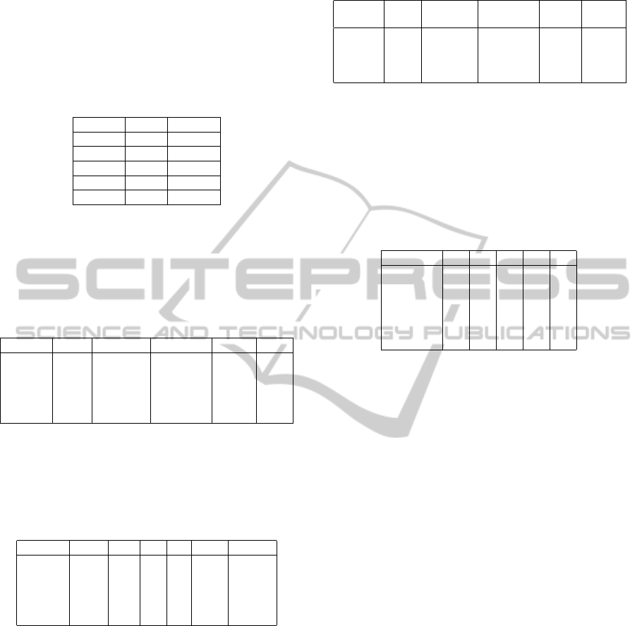
Let us show the result of our POS filter in table 3. As
the result says, recall factors go up to 70% (n = 3)
and no change arises any more. On the other hand,
precision goes down to 7 % at n = ∞.
Table 3: POS Filtering.
n-Xgram Recall Precision
2 71.8 26.7
3 76.1 23.1
4 76.1 12.1
5 76.1 10.1
∞ 76.1 7.2
Let us illustrate the numbers of frequent word sets
(co-occurrences) with each support in table 4. The
bigger n and the smaller support value we have, the
more word sets we have. This is because we must
have the more candidates at bigger n.
Table 4: Frequent Word Sets (Counts).
n-Xgram ∼ 0.1 0.1 ∼ 0.07 0.07∼ 0.04 0.04 ∼ Total
2 17 14 84 876 991
3 22 20 98 1241 1381
4 23 25 118 1515 1681
5 26 33 132 1715 1906
∞ 225 222 870 6346 7663
Table 5 shows how many words constitute one co-
occurrence in n-grams. Though we obtain many fre-
quent co-occurrenes, the average is 2.00 to 2.11 but
no co-occurrence of length.
Table 5: Length of Frequent words.
n-Xgram 2 3 4 5- Total AvgLen
2 991 - - - 991 2.00
3 1,292 90 - - 1382 2.07
4 1,503 165 13 - 1681 2.11
5 1,728 165 13 0 1906 2.10
∞ 7,485 165 13 0 7664 2.02
Table 6 contains the number of frequent word sets
obtained over n-Xgrams but not over (n −1)-Xgrams.
This shows that there happen huge amount of frequent
sets over ∞-Xgrams.
We illustrate all the frequencies of the cor-
rect collocations using the several features over
each n-Xgrams within the collections of top 50 co-
occurrences according to the feature values in table
7. Note we say ”correct” when the frequent word set
appears in dictionaries. For example, in CF (Top50),
we get 23 correct co-occurrences (collocations) over
2-Xgram among 50 co-occurrences, but 6 correct col-
locations over ∞-Xgrams. Generally we get the worse
precision at bigger n in every case, because there
Table 6: Newly Generated Sets (Counts).
n-Xgram ∼ 0.1 0.1 ∼ 0.07 0.07 ∼ 0.04 0.04 ∼ Correct
(Best)
2 - 3 2 2 3 358 8
3 - 4 0 1 1 272 4
4 - 5 0 0 0 200 0
5 - ∞ 2 9 202 4418 0
happen more and more frequent word sets. Since
we have extracted collocations of average 2.0-2.11
words, we’d better discuss cases over 2- or 3-Xgrams.
To our surprise, we get the more collocations in CF
Middle50 (Mid50), which means CF (Co-occurrence
Frequency) is not suitable since the higher CF doesn’t
correspond to the better result.
Table 7: Extracting Collocations (Counts) - Top50.
n-Xgram 2 3 4 5 ∞
CF 23 16 15 13 6
CF(Mid50) 29 19 20 11 10
PMI 42 36 36 31 33
DC 44 38 38 36 31
TS 42 35 32 27 17
PLL 34 30 26 23 7
Table 8 contains the comparison. For example, in
a case of CF with n=2 and Top10, we get 20 percent
correctness with the top 10 co-occurrences of CF val-
ues so that we have 0.2 ×10 = 2 collocations. In all
the cases, CF doesn’t work well. Since we have good
precision at 2-Xgrams in all the cases except CF, we
examine mainly the cases of n = 2 and n = 3. PMI
and DC work well in a case of 2-Xgram while TS and
PLL don’t. In fact, we get PMI and DC about 1.1 to
1.4 times better than TS and PLL. In n = 3, PMI and
DC show 1.1 to 1.2 better results compared to TS, but
1.0 to 1.25 worse than PLL. In n = 4,5 and ∞, we get
much better results about PMI, DC and PLL than TS.
In these cases, all of the Top50 values are comparable
with each other, which means TS gives many colloca-
tions not in the top range. In any cases, PLL doesn’t
work best but not really bad even in 5-Xgram. PLL
may capture some aspects of collocation properly.
4.3 Discussion
Let us discuss what our results mean. Clearly
POS filter works well because of recall 70% (ta-
ble 3). Although ∞-Xgram may capture much more
collocations in our corpus, we miss 30% of them.
The main reason comes from morphological analy-
sis and/or segmentation. For example, a proper noun
”gekidanshiki” was decomposed into two nouns as
”gekidan/shiki” (Theatre four-season) where both
are general nouns.
Since we missed about 30% n-Xgrams at POS fil-
MiningJapaneseCollocationbyStatisticalIndicators
385
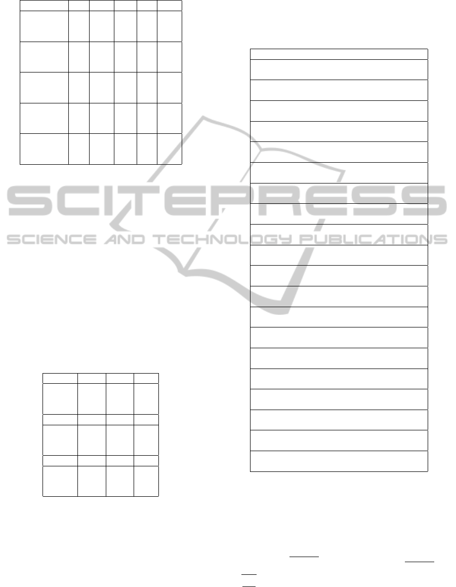
Table 8: Precision (%) in n-Xgram.
Feature CF PMI DC TS PLL
(n=2) Top10 20 100 100 70 70
Top20 30 90 95 80 65
Top50 46 84 88 84 68
(n=3) Top10 20 60 60 50 80
Top20 20 75 65 55 65
Top50 34 72 76 70 60
(n=4) Top10 20 80 60 40 70
Top20 15 80 65 40 70
Top50 32 72 76 64 52
(n=5) Top10 20 50 60 20 60
Top20 15 60 65 30 65
Top50 26 62 72 54 46
(n=∞) Top10 0 50 60 10 0
Top20 5 60 60 15 10
Top50 12 66 62 34 14
tering, we have examined the entire corpus by hand
to obtain (new) collocations. And we got 27 re-
sults, many of them come from different segmenta-
tion, word stems and POS filtering. Morphological
processing should be discussed in different ways.
As shown in a table 5, we have obtained co-
occurrences over 2-, 3- and 4-Xgrams. But there arise
few frequent word sets as in table 6 over 5- and ∞-
Xgrams. In fact, the average length is 2.00 to 2.11
and no co-occurrence with length 5 happens. It seems
that 2- and 3-Xgrams are enough to examine our col-
location. The right column of the table 6 shows, al-
though new frequent word sets are generated, few
correct ones (collocations) remain in the best support
case over 4-, 5- and ∞-Xgrams in the corpus.
Table 9: Cross Comparisons (Counts in 2-/3-Xgrams).
(Top10) DC TS PLL
PMI [6/7] 0/0 1/0
DC 1/0 0/0
TS 0/0
(Top20) DC TS PLL
PMI 12/14 1/0 4/1
DC 6/2 3/2
TS 0/0
(Top50) DC TS PLL
PMI 40/35 13/6 16/5
DC 23/17 15/6
TS 4/2
Let us compare the results by several features. In
2-Xgram, generally we get nice precisions of more
than 80 % in PMI, DC and TS even in Top50. In 3-
Xgram, both PMI and DC work better than TS and
PLL is not bad. Let us examine the differences shown
in a table 9 where each item shows how many co-
occurrences appear in two features.
We show Top20 results of 2-Xgrams with the fea-
tures (PMI,DC,TS and PLL) in tables 10, 11, 12 and
13 where an asterisk mark(*) means the item appears
also in Dice Coefficient table and a double asterisk
mark(**) means the item of Dice Coefficient table ap-
pears also in Pairwose Mutual Information table.
Table 10: Top20 on 2-Xgram (DC).
Co-occurrence / meaning : DC : Y/N
shuki(alcoholic smell) obiru(have)
be drunk : 0.755 : Y
mimi(ear) katamukeru(bend)
listen : 0.438 : Y*
hone(bone) oru(break)
make an effort : 0.347 : Y
tama(ball) furu(wave)
wave a ball : 0.320 : Y
nessen(close game) kurihirogeru(develop)
play exciting games : 0.317 : Y
shorui(document) sokensuru(send)
file charges : 0.293 : Y*
ase(sweat) nagasu(wash off)
work hard : 0.269 : Y
taicho(physical condition) kuzusu(destroy)
become ill : 0.251 : Y
kesho(slight wound) ou(receive)
slightly injured : 0.236 : Y**
kisha(journalist) kaikensuru(meet)
meet the press : 0.234 : Y**
sagi(fraud) furikomeru(transfer)
remittance fraud : 0.234 : N**
sake (sake) nomu(drink)
drink alcohol : 0.225 : Y**
alcohol(alcohol) kenshutsusuru(detect)
detect the influence of alcohol : 0.223 : Y
akushu(hand-shaking) kawasu(excahnge)
shake hands 0.220 : Y
garasu(glass) waru(break)
break glasses : 0.216 : Y
110ban(police) tsuhosuru(call)
call police : 0.215 : Y
genin(cause) shiraberu(investigate)
examine the cause 0.213 : Y**
jusho(serious illness) ou(suffer)
seriously injured : 0.209 : Y**
shindo(seismic intensity) kansokusuru(observe)
observe magnitude : 0.209 : Y
ashi(hoot) hakobu(carry)
come : 0.207 : Y**
For example, in a case of PMI and DC, we got
6 and 7 co-occurrences in 2-Xgram and 3-Xgram of
Top10 respectively. Since the precisions are 100%
and 60%, we have 6 × 1.00 = 6 and 7 × 0.60 =
4 collocations. Here we have many common co-
occurrences between PMI and DC. In fact, using
n
1
+ n
2
≥ 2
√
n
1
×n
2
, we see DC = 2 ×
n
12
n
1
+ n
2
≤
r
n
12
N
×2
PMI/2
. This means DC preserves ordering
by PMI if both n
1
and n
2
work equally and n
12
keeps
constant, i.e., DC depends on PMI and the number of
ICEIS2013-15thInternationalConferenceonEnterpriseInformationSystems
386
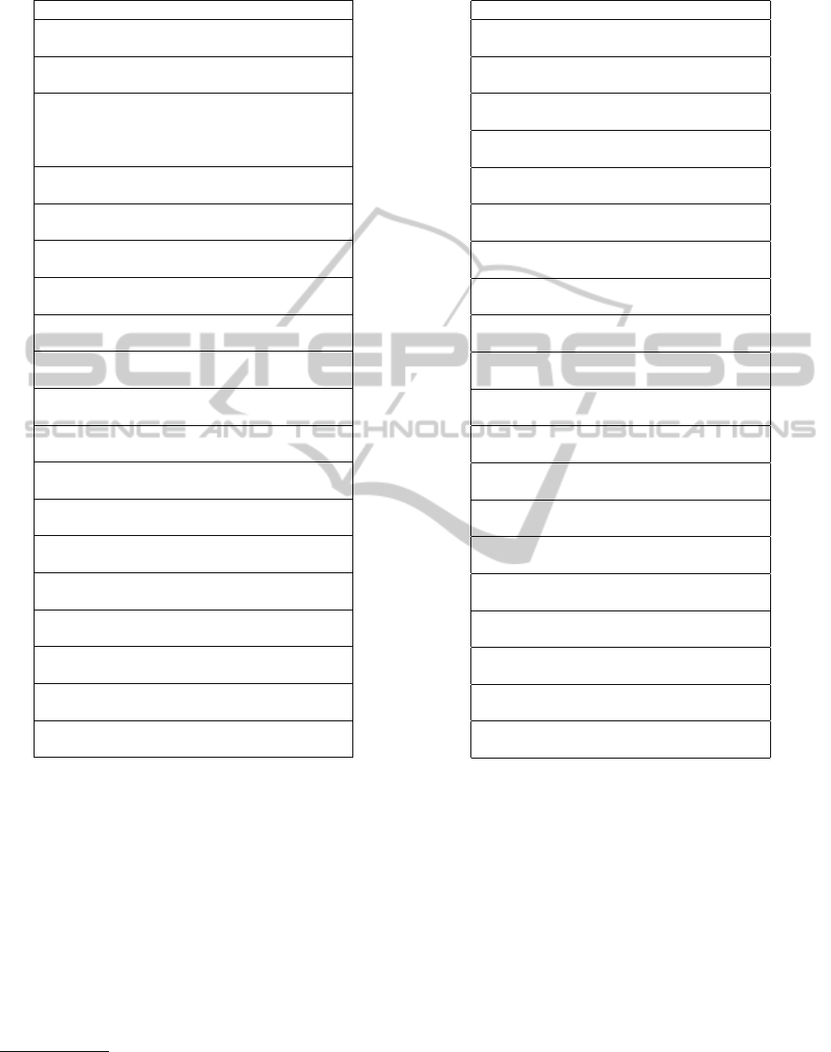
Table 11: Top20 on 2-Xgram (PMI).
Co-occurrence / meaning:PMI:Y/N
shuki(alcoholic smell) obiru(have)
be drunk : 10.3 : Y*
hone(bone) oru(break)
make an effort : 9.44 : Y*
mimi(ear) katamukeru(bend)
listen : 9.23 : Y*
taicho(physical condition) kuzusu(destroy)
become ill : 9.13 : Y*
akushu(hand-shaking) kawasu(excahnge)
shake hands : 8.83 : Y*
shindo(seismic intensity) kansokusuru(observe)
observe magnitude : 8.75 : Y*
nessen(close game) kurihirogeru(develop)
play exciting games : 8.63 : Y*
tama(ball) furu(wave)
wave a ball : 8.62 : Y*
kufu(device) korasu(elaborate)
exercise ingenuity : 8.44: Y
alcohol(alcohol) kenshutsusuru(detect)
detect the influence of alcohol : 8.43 : Y*
110ban(police) tsuhosuru(call)
call police : 8.35 : Y*
yozai(other crimes) tsuikyusuru(investigate)
investigate extra crimes : 8.24: Y
kagi(key) niguru(hold)
hold the key : 8.22: Y
ase(sweat) nagasu(wash off)
work hard : 8.21 : Y*
jusho(serious illness) oru(hurt)
hurt severely : 8.08 : N
teinen(retirement age) taishokusuru(leave)
retire : 8.03 : Y
kizu(wounds) saguru(investigate)
reopen woulds : 8.02 : Y
garasu(glass) waru(break)
break glasses : 7.95 : Y*
zenryoku(all the effort) tsukusu(exhaust)
do best : 7.93 : Y
kikin(fund) torikuzusu(reduce)
reduce fund : 7.69 : N
co-occurrences.
In Top50 of n=2, there arise 13 and 16 common
co-occurrences between PMI and TS and between
PMI and PLL respectively, but few between TS and
PLL (4 occurrences). Since the precisions are about
60% to 80%, the differences seem to come from the
one between TS and PLL.
In a table 14, we summarize the difference be-
tween TS and PLL in a case of Top50 and n=2,..,5, ∞.
We see few common co-occurrences arise although
all these are correct. Also more than half occurrences
in TS-PLL and PLL-TS are correct
6
. This means TS
6
Note TS-PLLmeans all the co-occurrences in TS but
not in PLL. In the table, 46and (39)mean there are 46 co-
occurrences and 39 are correct among them.
Table 12: Top20 on 2-Xgram (TS).
Co-occurrence / meaning : TS : Y/N
shirabe(investigation) yoru(according to)
according to the investigation : 74.1: Y
utagai(suspicion) taihosuru(arrest)
arrest on suspicion : 48.5: N
kisha(journalist) kaikensuru(meet)
meet the press : 47.9 : Y*
genin(cause) shiraberu(investigate)
examine the cause : 43.7 : Y*
genko( flagrante delicto) taihosuru(arrest)
catch red-handed : 42.4 : N
chikara(stress) ireru(lay)
emphasize : 41.6 : Y
yogi(suspicion) taihosuru(arrest)
arrest on suspicion : 40.6 : N
kangae(though) shimesu(show)
put ideas : 37.2 : Y
hito(person) iru(there exist)
there is a person : 36.2 : Y
koe(call) kakeru(shout)
cal out : 34.0 : Y
tsuyoi(hard) utsu(hit)
hit (a heart) strongly : 32.7 : Y
shuki(alcoholic smell) obiru(have)
be drunk : 32.6 : Y*
shorui(document) sokensuru(send)
file charges : 32.0 : Y*
egao(smile) miseru(show)
show a smile : 31.8 : Y
mi(body) tsukeru(put)
learn : 31.1 : Y
ashi(hoot) hakobu(carry)
come : 30.8 : Y*
tsumi(crime) tou(ask)
accuse of a crime : 30.0 : Y
kesho(slight wound) ou(receive)
slightly injured : 30.0 : Y*
hanashi(story) kiku(listen)
listen carefully : 29.6 : Y
eikyo(influence) ataeru(give)
affect : 29.5 : Y
and PLL extract different kinds of collocations from
PMI/DC.
5 CONCLUSIONS
In this investigation, we have proposed how to ex-
tract Japanese collocations by using data mining tech-
niques and statistical filters. To do that, we have pro-
posed POS filters, extended n-gram (n-Xgrams) as
well as several features. Then we have examined them
to extract collocations.
We have shown POS filters are useful, say 70 %
recall, and patterns not matching the filters depends
on morphological processing. We have also shown
MiningJapaneseCollocationbyStatisticalIndicators
387
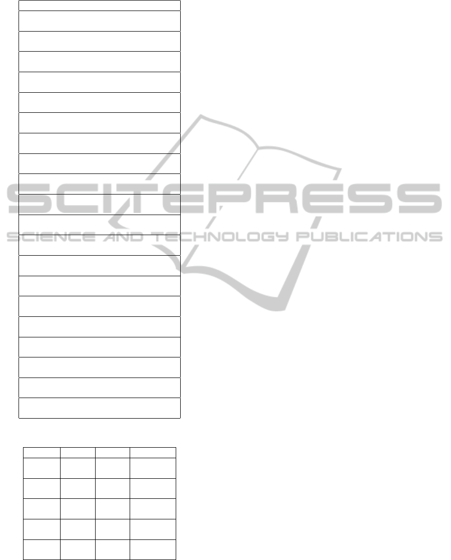
Table 13: Top20 on 2-Xgram (PLL).
Co-occurrence / meaning : PLL : Y/N
<PER> uketamawaru(receive)
be told : 2.33 : N
me(eye) hosomeru(narrow)
smile sweetly : 4.37 : Y
kikin(fund) torikuzusu(reduce)
reduce fund : 6.74 : N
sake(sake) you(be drunk)
get drunk : 6.81 : Y
kubi(neck) shimeru(strangle)
end up bringing ruin : 8.35 : Y
kufu(device) korasu(elaborate)
exercise ingenuity : 8.4 : Y
byoin(hospital) hansosuru(transport)
transport to a hospital : 8.68 : Y
eikyo(influence) oyobosu(give)
affect : 9.09 : Y
hana(flower) sakaseru(make bloom)
become successful : 9.31 : Y
choeki(penal servitude) kyukeisuru(demand)
demand a penal servitude : 11.22 : N
ki(feeling) hikishimeru(strain)
brace oneself : 12.01 : Y
taisaku(measure) kojiru(take)
take a measure : 12.75 : Y
chosa(survey) kikitoru(hear)
inquiry survey : 12.86 : N
sagi(fraud) furikomeru(transfer)
remittance fraud : 12.94 : N*
seikyu(request) kikyakusuru(reject)
reject a claim : 13.75 : N
hone(bone) oru(break)
make an effort : 14.68 : Y*
yogi(suspicion) hininsuru(deny)
deny the charge : 15.47 : N
chikara(power) sosogu(work)
do best : 16.13 : Y
mimi(ear) katamukeru(bend)
listen : 16.14 : Y*
hyojo(look) ukaberu(show)
have an expression : 16.32 : Y
Table 14: TS vs PLL(Counts in Top50).
n-Xgram TS-PLL PLL-TS TS and PLL
2 46 46 4
(39) (30) (4)
3 48 48 2
(34) (29) (2)
4 49 49 1
(31) (25) (1)
5 49 49 1
(26) (22) (1)
∞ 50 50 0
(17) (7) (0)
more than 5-Xgram are not really useful for the ex-
traction. Frequent word sets don’t always correspond
to collocation but we can expect 30-40 % precision.
We have shown PMI and DC are useful features, say
more than 80 % accuracy in Top20 using 2-Xgrams,
more than 70% in Top50 using 2-,3- and 4-Xgrams.
Another feature, PLL, shows more than 60% in Top20
using 2-,3-, 4- and 5-Xgrams. PMI and DC contain
many common co-occurrences, but few between TS
and PLL.
REFERENCES
Backhaus, A. (2006) Co-location of education as a unit of
vocabulary, Journal of International Student Center,
Hokkaido University (in Japanese)
Han, J. and Kamber, M. (2006) Data Mining (2nd ed.) Mor-
gan Kauffman, 2006
Harremoes, P. and Tusnady, G. (2012) Information Di-
vergence is more chi-squared distributed than the chi
squared statistic proc. ISIT 2012, pp. 538-543
Himeno, M. (2004) Kenkyu-Sha Nihongo Hyogen
Katsuyou Jiten (Dictionary of Japanese Notation)
Kenkyu-Sha (in Japanese), 2004
Ishikawa, S. (2000) Statistical Indexes for Identifying Col-
locations in Corpus Research Institure for Mathemat-
ical Sciences 190, pp. 1-28, 2006, Kyoto. Univ. (in
Japanese)
Justeson, J., Katz, S. (1995) Technical terminology: some
linguistic properties and an algorithm for identifica-
tion in text Natural Language Engineering, 1995
Kurohashi, S. and Nagao, M. (1994) A method of case
structure analysis for Japanese sentences based on ex-
amples in case frame dictionary. In IEICE Transac-
tions on Information and Systems, Vol. E77-D No.2,
1994 (in Japanese)
Manning, D. and Schutze,H. (1999) Foundations of Statis-
tical Natural Language Processing MIT Press, 1999
Sonoda, T. and Miura, T. (2012) Data Mining for Japanese
Collocation 7th International Conference on Digital
Information Management (ICDIM), Macau, 2012
Stubbs, M. (2002) Words and Phrases – Corpus Studies of
Lexical Semantics Blackwell Publishers, 2001
Tanomura, T. (2009) Retrieving collocational information
from Japanese corpora : An attempt towards the cre-
ation of a dictionary of collocations Osaka Univer-
sity Bulletin, Osaka University Knowledge Archive
(in Japanese), 2009
Yang, Y. and Pedersen, J.O. (1997) A Comparative Study
on Feature Selection in Text Categorization Proc. In-
ternational Conference on Machine Learning (ICML),
1997, pp.412-420
ICEIS2013-15thInternationalConferenceonEnterpriseInformationSystems
388
