
Parameterised Fuzzy Petri Nets for Knowledge Representation
and Reasoning
Zbigniew Suraj
Institute of Computer Science, University of Rzesz
´
ow, Rzesz
´
ow, Poland
Keywords:
Parameterised Fuzzy Petri Net, Production Rule, Knowledge Representation, Approximate Reasoning,
Rule-based System.
Abstract:
The paper presents a new methodology for knowledge representation and reasoning based on parameterised
fuzzy Petri nets. Recently, this net model has been proposed as a natural extension of generalised fuzzy Petri
nets. The new class extends the generalised fuzzy Petri nets by introducing two parameterised families of sums
and products, which are supposed to provide the suitable t-norms and s-norms. The nature of the fuzzy reason-
ing realised by a given net model changes variously depending on t- and/or s-norms to be used. However, it is
very difficult to select a suitable t- and/or s-norm function for actual applications. Therefore, we proposed to
use in the net model parameterised families of sums and products, which nature change variously depending
on the values of the parameters. Taking into account this aspect, we can say that the parameterised fuzzy
Petri nets are more flexible than the classical fuzzy Petri nets, because they allow to define the parameterised
input/output operators. Moreover, the choice of suitable operators for a given reasoning process and the speed
of reasoning process are very important, especially in real-time decision support systems. Some advantages
of the proposed methodology are shown in its application in train traffic control decision support.
1 INTRODUCTION
A substantial share of currently developed IT systems
is based on knowledge often represented in the form
of a decision rule system. Knowledge can be acquired
either from experts directly, in the course of an IT sys-
tem’s implementation or automatically from properly
processed training data. The knowledge combined
with an appropriate inference engine serves as a fun-
damental component of, among others, decision sup-
port systems. The steady growth in the number of IT
systems’ applications contributes greatly to the devel-
opment of systems capable of processing larger and
larger data amounts with major constraints related to
time limits in decision making. In response to the IT
system market, numerous scientific initiatives are un-
dertaken whose main aim is to either improve exist-
ing or launch new methods supporting development
of systems with knowledge base that could fulfill all
requirements. Most of all, new methods of knowledge
representation are being searched these days, as well
as knowledge quality verification or knowledge cod-
ing methods during implementation of decision sup-
port systems. A key feature of the methods is their
ability to verify quality of any rule system at the earli-
est possible stage of its development. The early fault
detection is crucial for economic reasons, such as al-
lowing cost reduction of the system’s development.
Moreover, it is also for the sake of the final product’s
quality, as errors identified and excluded at early de-
velopment stages, are not transferred to the successive
ones (Avram, 2005),(Jackson, 1999).
In the last years we can observe growing inter-
est in the design and exploitation of decision sup-
port systems built on the basis of uncertain knowl-
edge. In this way various methods of knowledge
representation and reasoning have already been pro-
posed. One of the most popular approaches to knowl-
edge representation are the fuzzy production rules.
They are often presented in the form of IF-THEN.
One of its benefits is that they create a modular and
well-structured knowledge base. Moreover, the rule
knowledge representation is quite natural and allows
for an easy understanding and tracing the reasoning
process. Nevertheless, there is much need and interest
in improving the existing solutions in this area. Hu-
man decision-making power is mainly based on rea-
soning and decision-making in an uncertain environ-
ment, where only imprecise, incomplete, and vague
information is available. This functional feature of
5
Suraj Z..
Parameterised Fuzzy Petri Nets for Knowledge Representation and Reasoning.
DOI: 10.5220/0004403000050013
In Proceedings of the 2nd International Conference on Data Technologies and Applications (DATA-2013), pages 5-13
ISBN: 978-989-8565-67-9
Copyright
c
2013 SCITEPRESS (Science and Technology Publications, Lda.)

knowledge-based systems should be taken into ac-
count in the course of their creation. In this field of
research, the representation of uncertain information
and the ability to draw conclusions from suppositions
contribute to a major research challenge (Dubois and
Prade, 1996). The fuzzy set theory has emerged as a
powerful means to describe and deal with that kind of
uncertainty (Zadeh, 1965),(Zimmermann, 1993).
For further improvement of the implementation of
large knowledge bases, a graphical representation of
the rule base is desirable. Petri nets are a suitable
graphical and mathematical means of description for
this purpose. For relatively long time, Petri nets have
been very popular among people specialised in Artifi-
cial Intelligence due to the nets’ adequacy to represent
an approximate process as a dynamic discrete event
system (Cardoso and Camargo, 1999).
The concept of a fuzzy Petri net has its origin in
C.G. Looney’s article (Looney, 1988). In the last four
decades, many extensions of Petri nets or their modifi-
cations have been proposed (Chen et al., 1990),(Fryc
et al., 2004a),(Fryc et al., 2004b),(Pedrycz and Go-
mide, 1994),(Pedrycz and Peters, 1998),(Peters et al.,
1998),(Suraj, 2012a),(Suraj, 2012b),(Suraj, 2012c).
The paper presents a new methodology for knowl-
edge representation and reasoning based on param-
eterised fuzzy Petri nets (in short PFPNs) (Suraj,
2012c). Recently, this net model has been proposed
as a natural extension of generalised fuzzy Petri nets
(Suraj, 2012a). The new class extends the gener-
alised fuzzy Petri nets by introducing two parame-
terised families of sums and products, which are sup-
posed to provide the suitable t-norms and s-norms.
In particular, this paper provides a method for
knowledge representation as well as an algorithm for
construction of a PFPN model on the base of a given
set of fuzzy production rules. The proposed method-
ology is not only more convenient in terms of knowl-
edge representation, but most of all it is more effective
in the modelling of reasoning process as in the new
class of fuzzy Petri nets the user has the chance to
define the parameterised input/output operators. The
choice of suitable operators for a given reasoning pro-
cess and the speed of reasoning process are very im-
portant, especially in real-time decision support sys-
tems.
The structure of this paper is as follows. In Sect.
2 we give a brief introduction to triangular norms, pa-
rameterised families of sums and products, and PF-
PNs. Sect. 3 describes transformations of produc-
tion rules into PFPNs. In Sect. 4 we present two al-
gorithms. The first algorithm allows to construct the
PFPN model based on a set of production rules in an
automatic way. The second one describes a reasoning
process modelled by means of a given PFPN. An ex-
ample illustrating the performance of this algorithm
is given in Sect. 5. Sect. 6 includes remarks on di-
rections for further research related to the presented
methodology.
2 PRELIMINARIES
In this section, basic notions and notation (especially
concerning PFPNs (Suraj, 2012c)) used in the pro-
duction rule representation and reasoning based on
PFPNs are recalled.
2.1 Triangular Norms
and their Families
Basic operations in the fuzzy set theory such as the in-
tersection and the union, are defined by using the min-
imum and maximum functions. However, some other
definitions of these operations are often employed,
too. In particular, for the intersection and the union t-
norms and s-norms are often used. As the t-norms and
s-norms are also used for defining PFPNs, we recall
their definitions (Fedrizzi and Kacprzyk, 1999),(Kle-
ment et al., 2000).
Let [0, 1] be the closed interval of all real numbers
from 0 to 1 (0 and 1 are included).
A t-norm is defined as t : [0, 1] × [0, 1] → [0, 1]
such that, for each a, b, c ∈ [0, 1]: (1) it has 1 as the
unit element, i.e., t(a, 1) = a; (2) it is monotone,
i.e., if a ≤ b then t(a, c) ≤ t(b, c); (3) it is commu-
tative, i.e., t(a, b) = t(b, a); (4) it is associative, i.e.,
t(t(a, b), c) = t(a, t(b, c)).
More relevant examples of t-norms are: the min-
imum t(a, b) = min(a, b) used most widely, the alge-
braic product t(a, b) = a ∗ b, the Łukasiewicz t-norm
t(a, b) = max(0, a + b −1).
An s-norm (or a t-conorm) is defined as s : [0, 1] ×
[0, 1] → [0, 1] such that, for each a, b, c ∈ [0, 1]: (1)
it has 0 as the unit element, i.e., s(a, 0) = a, (2) it
is monotone, i.e., if a ≤ b then s(a, c) ≤ s(b, c), (3)
it is commutative, i.e., s(a, b) = s(b, a), and (4) it is
associative, i.e., s(s(a, b), c) = s(a, s(b, c)).
More relevant examples of s-norms are: the maxi-
mum s(a, b) = max(a, b) used most widely, the prob-
abilistic sum s(a, b) = a + b − a ∗ b, the Łukasiewicz
s-norm s(a, b) = min(a + b,1).
There has been some intensive research in the
field of logical operators carried out for the last three
decades, which involves the development of parame-
terised families of sums and products. In Tables 1-2
exemplary lists of parameterised families of sums and
DATA2013-2ndInternationalConferenceonDataManagementTechnologiesandApplications
6

Table 1: An exemplary list of parameterised families of
sums.
Sum S(a,b,v) Range v
a+b−(2−v)∗a∗b
1−(1−v)∗a∗b
(0, ∞)
1 − [max(0, (1 − a)
−v
+ (1 − b)
−v
− 1)]
−1
v
(−∞, ∞)
a+b−a∗b−min(a,b,1−v)
max(1−a,1−b,v)
(0, 1)
1 − log
v
[1 +
(v
1−a
−1)(v
1−b
−1)
v−1
(0, ∞)
min[1, (a
v
+ b
v
)
1
v
(0, ∞)
1
1+[(
1
a
−1)
−v
+(
1
b
−1)
−v
]
−1
v
(0, ∞)
Table 2: An exemplary list of parameterised families of
products.
Product T(a,b,v) Range v
a∗b
v+(1−v)∗(a+b−a∗b)
(0, ∞)
[max(0, a
−v
+ b
−v
− 1)]
−1
v
(−∞, ∞)
a∗b
max(a,b,v)
(0, 1)
log
v
[1 +
(v
a
−1)(v
b
−1)
v−1
(0, ∞)
1 − min[1, ((1 − a)
v
+ (1 − b)
v
)
1
v
] (0, ∞)
1
1+[(
1
a
−1)
v
+(
1
b
−1)
v
]
1
v
(0, ∞)
products are presented. For more details one shall re-
fer to (Klement et al., 2000).
It is easy to observe that for the first elements of
Tables 1 and 2, and the parameter v = 1 we obtain the
probabilistic sum and the algebraic product, respec-
tively.
2.2 Parameterised Fuzzy Petri Nets
Now we recall the definition of PFPNs and their in-
terpretation in the field of decision support systems.
We assume that the reader is familiar with the ba-
sic notions of classical Petri nets (Peterson, 1981).
A parameterised fuzzy Petri net (PFP-net) is a tu-
ple (Suraj, 2012c):
N = (P, T, S, I, O, α, β, γ, Op, δ, M0),
where:
1. P = {p
1
, . . . , p
n
} is a finite set of places, n > 0;
T = {t
1
, . . . ,t
m
} is a finite set of transitions, m > 0;
S = {s
1
, . . . , s
n
} is a finite set of statements; the
sets P, T , S are pairwise disjoint and card(P) =
card(S), where card(X) denotes the number of el-
ements in a set X;
2. I : T → 2
P
is the input function, a mapping from
a set of transitions to a family of all subsets of the
set P; O : T → 2
P
is the output function, a mapping
from a set of transitions to a family of all subsets
of the set P;
3. α : P → S is the statement binding function, a bi-
jective mapping from a set of places to a set of
statements; β : T → [0, 1] is the truth degree func-
tion, a mapping from a set of transitions to [0,1];
γ : T → [0, 1] is the threshold function, a map-
ping from a set of transitions to [0,1]; Op is a
finite set of parameterised families of sums and
products called the set of parameterised opera-
tors; δ : T → Op × Op × Op is the operator bind-
ing function, a mapping from a set of transitions to
a set of all triples of parameterised operators from
the set of parameterised operators Op;
4. M0 : P → [0, 1] is the initial marking, a mapping
from a set of places to [0,1].
As for the graphical interpretation, places are de-
noted by circles and transitions by rectangles. The
function I describes the oriented arcs connecting
places with transitions, and the function O describes
the oriented arcs connecting transitions with places.
If I(t) = {p} then a place p is called an input place
of a transition t, and if O(t) = {p
0
}, then a place p
0
is called an output place of t. The initial marking M0
is an initial distribution of real numbers in the places.
It can be represented by a vector of dimension n of
real numbers from [0, 1]. For p ∈ P, M0(p) can be
interpreted as a truth value of the statement s bound
with a given place p by means of the binding function
α, i.e., α(p) = s. We assume that if the truth value
of a statement attached to a given place is equal to 0
then the token does not exist in the place. The number
β(t) is interpreted as the truth degree of an implication
(a rule) corresponding to a given transition t (Chen
et al., 1990),(Fryc et al., 2004b). The meaning of the
threshold function γ is explained below. The opera-
tor binding function δ connects transitions with triples
of parameterised operators (In
v
, Out
v
1
, Out
v
2
). The first
operator in this triple is called the input parameterised
operator, and two remaining ones are called the out-
put parameterised operators. The input parameterised
operator In
v
belongs to one of the parameterised fam-
ilies of sums and products. It concerns the way in
which all input places are connected to a given tran-
sition t (more precisely, statements corresponding to
those places). Moreover, the output parameterised op-
erator Out
v
1
belongs to the parameterised families of
products and Out
v
2
belongs to the parameterised fami-
lies of sums. Both of them concern the way in which
the marking is computed after firing the transition t.
This issue is explained more precisely below.
The PFPN dynamics defines how new markings
are computed from the current marking when transi-
tions are fired.
Let N be a PFP-net. A marking of N is a function
M : P → [0, 1].
ParameterisedFuzzyPetriNetsforKnowledgeRepresentationandReasoning
7

Let N = (P, T, S, I, O, α, β, γ, Op, δ, M0) be a PFP-
net, t ∈ T , I(t) = {p
i1
, . . . , p
ik
} be a set of input places
for a transition t, β(t) be a value of the truth degree
function β corresponding to t and β(t) ∈ (0, 1], γ(t)
be a value of threshold function γ corresponding to t,
M be a marking of N, and v be a parameter value for
a parameterised family of sums and products. More-
over, let In
v
be an input parameterised operator and
Out
v
1
, Out
v
2
be output parameterised operators with a
parameter value v corresponding to t.
A transition t ∈ T is enabled for marking M and a
parameter value v, if the value of parameterised input
operator In
v
for the transition t is positive and greater
than, or equal to, the value of threshold function γ cor-
responding to t and the parameter value v, i.e.,
In
v
(M(p
i1
), . . . , M(p
ik
)) ≥ γ(t) > 0
for p
i j
∈ I(t) and j = 1, . . . , k.
In the paper we consider two modes for firing tran-
sitions.
(Mode 1) If M with a parameter value v is a marking
of N enabling a transition t and M
0
v
the marking de-
rived from M with v by firing t, then for each p ∈ P:
M
0
v
(p) =
1. 0 if p ∈ I(t),
2. Out
v
2
(Out
v
1
(In
v
(M(p
i1
), . . . , M(p
ik
)), β(t)), M(p))
if p ∈ O(t),
3. M(p) otherwise.
In this mode, a procedure for computing the mark-
ing M
0
v
is as follows: (1) Numbers from all input
places of the transition t are removed (the first con-
dition from M
0
v
definition). (2) Numbers in all out-
put places of t are modified in the following way: at
first the value of a parameter value v is set, then the
value of parameterised input operator In
v
for all in-
put places of t is computed, next the value of param-
eterised output operator Out
v
1
for the value of In
v
and
for the value of truth degree function β(t) is deter-
mined, and finally, the value corresponding to M
0
v
(p)
for each p ∈ O(p) is obtained as a result of parame-
terised output operator Out
v
2
for the value of Out
v
1
and
the current marking M(p) (the second condition from
M
0
v
definition). (3) Numbers in the remaining places
of net N are not changed (the third condition from M
0
v
definition).
(Mode 2) If M with a parameter value v is a marking
of N enabling transition t and M
0
v
the marking derived
from M with v by firing t, then for each p ∈ P:
M
0
v
(p) =
1. Out
v
2
(Out
v
1
(In
v
(M(p
i1
), . . . , M(p
ik
)), β(t)), M(p))
if p ∈ O(t),
2. M(p) otherwise.
The main difference in the definition of the marking
M
0
v
presented above (Mode 2) concerns input places of
the fired transition t. In Mode 1 numbers are removed
from all input places of the fired transition t (c f . the
first definition condition of Mode 1), whereas in Mode
2 all numbers are copied from input places of the fired
transition t (the second definition condition of Mode
2).
Let us consider a PFPN in Figure 1(a). For the
net we have: the set of places P = {p
1
, p
2
, p
3
, p
4
, p
5
},
the set of transitions T = {t
1
,t
2
}, the set of statements
S = {s
1
, s
2
, s
3
, s
4
, s
5
}, the input function I and the out-
put function O in the form: I(t
1
) = {p
1
, p
2
}, I(t
2
) =
{p
2
, p
3
}, O(t
1
) = {p
4
}, O(t
2
) = {p
5
}. Moreover,
there are: the statement binding function α : α(p
1
) =
s
1
, α(p
2
) = s
2
, α(p
3
) = s
3
, α(p
4
) = s
4
, α(p
5
) = s
5
,
the truth degree function β: β(t
1
) = 0.7, β(t
2
) = 0.8,
the threshold function γ: γ(t
1
) = 0.4, γ(t
2
) = 0.3, the
set of parameterised operators Op = {S(.), T (.)} and
the operator binding function δ defined as follows:
δ(t
1
) = (S(.), T (.), S(.)), δ(t
2
) = (T (.), T (.), S(.)) with
a relevant parameter value v, and the initial marking
M0 = (0.6, 0.4, 0.7, 0, 0).
(a)
(b)
Figure 1: (a) A PFPN with the initial marking before firing
the enabled transitions t
1
and t
2
. (b) An illustration of a
firing rule: the marking after firing t
1
, where t
2
is disabled
(Mode 1).
If we take, for instance, the first parameterised
family of sums S(a, b, v) from Table 1, the first pa-
rameterised family of products T (a, b, v) from Ta-
ble 2 and a parameter value v = 1, then S(a, b, 1) =
a + b − a ∗ b and T (a, b, 1) = a ∗ b. For the transition
DATA2013-2ndInternationalConferenceonDataManagementTechnologiesandApplications
8
t
1
we have S(0.6, 0.4, 1) = 0.6+0.4−0.6 ∗ 0.4 = 0.76
and T (0.76, 0.7, 1) = 0.76 ∗ 0.7 = 0.53 by the initial
marking M0 and v = 1. As the global value for all
input places of t
1
and v = 1 equals 0.76, it is posi-
tive and greater than γ(t
1
) = 0.4. Thus, the transition
t
1
is enabled by M0 and v = 1. Firing transition t
1
by the marking M0 and v = 1 according to Mode 1
transforms M0 to the marking M
0
1
= (0, 0, 0.7, 0.53, 0)
(Figure 1(b)). It is easy to check that by the initial
marking M0 and v = 1 the transition t
2
is not enabled.
For more detailed information about PFPNs the
reader is referred to (Suraj, 2012c).
3 NET REPRESENTATION
OF PRODUCTION RULES
Now, we present a method of transforming rules into
a PFPN depending on the form of a transformed rule.
By using a PFPN, a basic rule (Type 0) of the
form:
IF s
j
THEN s
k
(CF = q
i
)
can be modelled as shown in Figure 2(a). The value of
a certainty factor (CF) is q
i
∈ [0, 1]. It represents the
reliability degree of the rule. The larger value q
i
, the
more credible the rule. Similarly, the value r
i
∈ [0, 1]
and represents the threshold value. Larger value of r
i
requires greater truth degree of the rule precedence,
i.e., s
j
. However, the operator In
v
, and the operators
Out
v
1
, Out
v
2
represent the parameterised input operator
and the parameterised output operators, respectively.
They play an important role in a description of rule
firing.
(a)
(b)
Figure 2: A PFPN representation of rule type 0: (a) before
firing t
i
, (b) after firing t
i
.
According to Figure 2(b) the value in an output
place p
k
of a transition t
i
corresponding to the rule is
calculated as
y
k
= Out
v
1
(y
j
, q
i
).
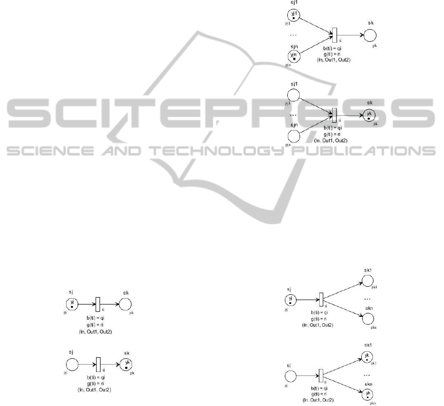
If the premise or the conclusion of a production
rule contains AND or OR (classical propositional
connectives), it is called a composite production rule.
Below, there types of composite production rules
are discussed:
Type 1: IF s
j1
AND(OR) . . . AND(OR) s
jn
THEN s
k
(CF = q
i
). This rule type can be modelled by a PFPN
as shown in Figure 3(a). The value is calculated in the
output place as follows (Figure 3(b)):
y
k
= Out
v
1
(In
v
(y
j1
, . . . , y
jn
), q
i
).
(a)
(b)
Figure 3: A PFPN representation of rule type 1: (a) before
firing t
i
, (b) after firing t
i
.
Type 2: IF s
j
THEN s
k1
AND .. . AND s
kn
(CF = q
i
).
This rule type can be modelled by a PFPN as shown
in Figure 4(a). The value is calculated in each output
place as follows (Figure 4(b)):
y
k
= Out
v
1
(y
j
, q
i
).
(a)
(b)
Figure 4: A PFPN representation of rule type 2: (a) before
firing t
i
, (b) after firing t
i
.
Type 3: IF s
j
THEN s
k1
OR . . . OR s
kn
(CF = q
i
).
Due to the fact that this rule type does not describe
any specific implication, we do not consider it in the
paper.
ParameterisedFuzzyPetriNetsforKnowledgeRepresentationandReasoning
9

Remarks:
1. Due to technical reasons the names of functions
β, γ in Figures 2-4 are represented by b and g,
respectively.
2. Similarly, the parameter v appearing in the opera-
tors In
v
, Out
v
1
and Out
v
2
in Figures 2-4 is omitted.
3. As rule Types 0 and 2 have only one statement
in their premises, we may omit the input param-
eterised operator In
v
in Figures 2 and 4. Never-
theless, for better readability of these figures we
leave the operator where it is.
4. We assume that the initial markings of output
places are equal to 0 in all net models correspond-
ing to the considered rule types. Therefore, in
the descriptions of the values in output places we
do not regard the parameterised output operator
Out
v
2
. In the opposite case, i.e., for non-zero mark-
ings of output places, we should take into account
this parameterised output operator. Thus, in each
formula presented above the final value y
0
k
should
be computed as follows:
y
0
k
= Out
v
2
(y
k
, M(p)),
where y
k
denotes the values computed for suitable
rule types by means of formulas presented above,
and M(p) is a marking of output place p. Intu-
itively, a final value corresponding to M
0
v
for each
p ∈ O(p) is obtained as a result of Out
v
2
opera-
tion for the computed Out
v
1
operation value and
the current marking M(p) (the first/second condi-
tion depending on the firing mode from M
0
v
defi-
nition, Subsect. 2.2).
4 ALGORITHMS
4.1 Knowledge Representation
This section presents an algorithm for constructing a
PFPN on the base of a given set of production rules.
Algorithm 1: A construction of PFPN.
Input: A finite set R of production rules.
Output: A PFP-net N.
begin
F :=
/
0;
foreach r ∈ R do
begin
if r is a rule of Type 0 then Construct a subnet
N
r
as shown in Figure 2(a)
else if r is a rule of Type 1 then Construct
a subnet N
r
as shown in Figure 3(a)
else if r is a rule of Type 2 then Construct
a subnet N
r
as shown in Figure 4(a);
F := F ∪{N
r
};
end;
Integrate all subnets from a family F on joint
places and create a result net N;
return N;
end.
Notice: The symbol := denotes the assignment oper-
ator.
The input for this algorithm is a set of given pro-
duction rules R, whereas the output is a PFP-net N.
We can divide operating of the algorithm into two
phases. In the first phase the algorithm constructs
a suitable subnet N
r
depending on the rule type de-
scribed in Sect. 3. In the second one it creates a struc-
ture of a result net N integrating the constructed sub-
nets on joint places, i.e., places with which the same
statements appearing in different rules are associated.
In order to obtain a PFPN serving as the net model
of the approximate process described by production
rules from the set R, an initial marking corresponding
to the given statement truth values should be added to
the result net.
4.2 Approximate Reasoning
In many situations we may want to determine the
antecedent-consequence relationships between two
groups of statements: the starting (given) state-
ments s
i1
, . . . , s
ik
, and goal (computed) statements
s
o1
, . . . , s
ol
. In the Petri net representation, the places
associated with the first group of statements are called
starting places, whereas places associated with the
second one are called goal places. Furthermore, if
the truth degrees of starting statements s
i1
, . . . , s
ik
are
given, we may want to know what the truth degrees
of the goal statements s
o1
, . . . , s
ol
are. These problems
can be solved by using an approximate reasoning al-
gorithm based on PFPNs.
We assume that the truth degrees of starting state-
ments are given by the expert or they are identified by
sensors in finite time units. The goal of reasoning is
to determine the truth degrees of output (goal) state-
ments.
Algorithm 2: A description of approximate reasoning pro-
cess.
Input: The initial marking of starting places.
Output: The final marking of goal places.
begin
while It is not the end of the simulation do
DATA2013-2ndInternationalConferenceonDataManagementTechnologiesandApplications
10

begin
Determine transitions enabled for firing;
while There is a transition enabled for firing do
begin
Compute a new marking of all places after
firing the transition;
Determine a new transition enabled for
firing;
end;
Read the final marking of goal places;
Reset the final marking of all places;
end;
end.
Algorithm 2 can be performed in two different
modes corresponding to Mode 1 or Mode 2 described
in section 2.2. After firing a given transition (rule)
in Mode 1, tokens from its input places are removed.
Firing a given transition (rule) and removing tokens
can be intuitively interpreted as an execution of rea-
soning by using this rule in a given reasoning process.
Hence in the next steps, markings of input places of a
fired rule are already unnecessary. Such reasoning can
be understood as a kind of forward reasoning. How-
ever, in Mode 2 after firing a given transition (rule),
tokens remain in its input places. Contrary to Mode 1,
this way of firing rules can be applied to the systems
for which some statements appear in antecedents of
several rules fired in different reasoning steps. In the
following section we present an example of these two
algorithms’ use.
5 ILLUSTRATING EXAMPLE
In order to illustrate the simplicity and the power of
our methodology, let us show an application of the
algorithms described in Sect. 4 in the domain of train
traffic control.
We consider the following situation: a train B
waits at a certain station for a train A to arrive in order
to allow some passengers to change train A to train B.
Now, a conflict arises when the train A is late. In this
situation, the following alternatives can be taken into
consideration:
1. Train B waits for train A to arrive. In this case,
train B will depart with delay.
2. Train B departs in time. In this case, passengers
disembarking train A have to wait for a later train.
3. Train B departs in time, and an additional train is
employed for the train A
0
s passengers.
To make a decision, several inner conditions have
to be taken into account, for example: the delay pe-
riod, the number of passengers changing trains, etc.
The discussion regarding an optimal solution to the
problem of divergent aims such as: minimisation of
delays throughout the traffic network, warranty of
connections for the customer satisfaction, efficient
use of expensive resources, etc. is disregarded at this
point.
In order to describe the traffic conflict, we propose
to consider the following set R of three rules:
1. IF s
2
OR s
3
THEN s
6
(CF = 0.8)
2. IF s
1
AND s
4
AND s
6
THEN s
7
(CF = 0.7)
3. IF s
4
AND s
5
THEN s
8
(CF = 0.9)
where: s
1
: ’Train B is the last train in this direction
today’, s
2
: ’The delay of train A is huge’, s
3
: ’There
is an urgent need for the track of train B’, s
4
: ’Many
passengers would like to change for train B’, s
5
: ’The
delay of train A is short’, s
6
: ’(Let) train B depart ac-
cording to schedule’, s
7
: ’Employ an additional train
C (in the same direction as train B)’, and s
8
: ’Let train
B wait for train A’.
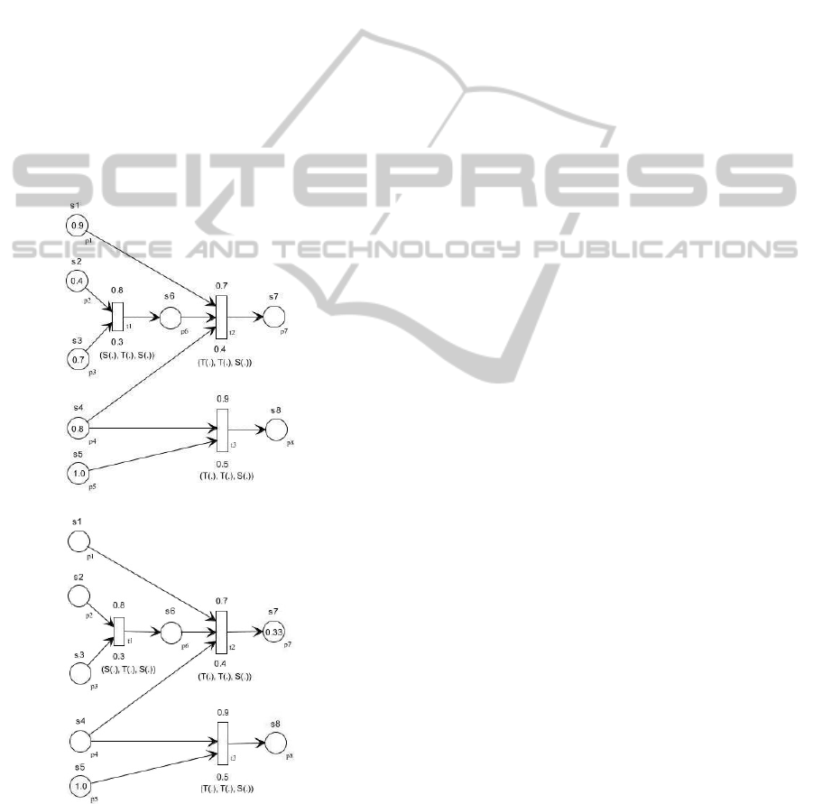
Applying the algorithm 1 from Sect. 4 to the set
R of rules together with their parameters we obtain
the PFP-net N corresponding to these rules shown in
Figure 5(a), where the logical operators OR, AND are
interpreted as the probabilistic sum S(·) and the al-
gebraic product T (·), respectively. Moreover, we as-
sume that the threshold value of these rules is equal
to 0.3, 0.4 and 0.5, respectively. Note that the places
p
1
, p
2
, p
3
and p
4
include the fuzzy values 0.9, 0.4,
0.7 and 0.8 corresponding to the statements s
1
, s
2
, s
3
and s
4
, respectively. In this example, the statement
s
5
attached to the place p
5
is the only crisp one and
its value is equal to 1. Moreover, we assume that the
set of parameterised operators Op = {S(.), T (.)} and
the operator binding function δ is defined as in Figure
5(a). Assessing the statements attached to the places
from p
1
up to p
5
, we observe that the transitions t
1
and t
3
can be fired. Firing these transitions according
to the firing rules for the PFPN model allows compu-
tation of the support for the alternatives in question.
In this way, the possible alternatives are ordered with
regard to the preference they achieve from the knowl-
edge base. This order forms the basis for further ex-
aminations and simulations and, ultimately, for the
dispatching proposal. If one chooses a sequence of
transitions t
1
t
2
they obtain the final value, correspond-
ing to the statement s
7
, equal to 0.33 (Figure 5(b)). In
the other case (i.e., for the transition t
3
only), the fi-
nal value, this time corresponding to the statement s
8
,
equals 0.72.
If we interpret the logical operators OR, AND as
the Łukasiewicz s-norm and Łukasiewicz t-norm, re-
spectively, and if we choose a sequence of transitions
t
1
t
2
then the final value is not possible to obtain. Af-
ParameterisedFuzzyPetriNetsforKnowledgeRepresentationandReasoning
11
ter firing the transition t
1
by the initial marking M0
we obtain the result marking by which the transition
t
2
is not able to fire. In the other case, i.e., for the tran-
sition t
3
, we obtain the final value for the statement s
8
equal to 0.7.
This example shows that different interpretations
for the logical operators OR and AND may lead to
quite different decision results. Therefore, we pro-
pose a new fuzzy net model in the paper, which is
more flexible than the classical one as in the former
class the user has the chance to define both the param-
eterised input/output operators. Chosing a suitable
interpretation for logical operators OR and AND we
may apply the mathematical relationships between t-
norms and s-norms or their families presented e.g. in
(Klement et al., 2000). The rest in this case certainly
depends on the experience of the model designer to a
significant degree. We omit this aspect of considera-
tions with respect to a limited space of the paper.
(a)
(b)
Figure 5: (a) An example of the PFPN model of train traffic
control. (b) An illustration of a firing rule: the marking after
firing a sequence of transitions t
1
t
2
(Mode 1).
6 CONCLUSIONS
In this paper, we have proposed a new methodology
for knowledge representation and reasoning based
on PFPNs. In particular, we have also provided
two algorithms supporting the proposed methodol-
ogy. These algorithms have been implemented in an
experimental application called PNES which supports
our methodology. This application has been devel-
oped on IBM PC, in Java. PNES consists of an editor
and a simulator. The editor allows inputting, editing
and selecting the values of the parameters for PFPNs
while the simulator starts with a given initial marking
and executes enabled transitions visualising reached
markings. Thanks to parallel firing rules correspond-
ing to transitions in a net representation we can speed
up an approximate process.
The proposed methodology has proved to be very
suitable for the design and implementation of a de-
cision support system in an exemplary problem with
relatively high practical relevance.
In our further investigations we will consider the
use of new classes of fuzzy Petri nets for inhibitory
rule representation (Delimata et al., 2009). Another
interesting problem arises while choosing relevant pa-
rameterised families of sums and products for actual
applications. These are examples of problems we
wish to examine exploring the approach presented in
the paper.
ACKNOWLEDGEMENTS
The author is grateful to the anonymous referees for
their helpful comments.
REFERENCES
Avram, G. (2005). Empirical study on knowledge based
systems. The Electronic Journal of Information Sys-
tems Evaluation, 8(1):11–20.
Cardoso, J. and Camargo, H., editors (1999). Fuzziness in
Petri Nets, volume 22 of Studies in Fuzziness and Soft
Computing. Physica-Verlag, Berlin.
Chen, S., Ke, J., and Chang, J. (1990). Knowledge represen-
tation using fuzzy petri nets. IEEE Trans. on Knowl-
edge and Data Engineering, 2(3):311–319.
Delimata, P., Moshkov, M., Skowron, A., and Suraj, Z.
(2009). Inhibitory Rules in Data Analysis. A Rough
Set Approach. Springer, Berlin.
Dubois, D. and Prade, H. (1996). What are fuzzy rules and
how to use them. Fuzzy Sets and Systems, 84:169–
185.
DATA2013-2ndInternationalConferenceonDataManagementTechnologiesandApplications
12

Fedrizzi, M. and Kacprzyk, J. (1999). A brief introduction
to fuzzy sets and fuzzy systems. In Cardoso, J. and Ca-
margo, H., editors, Fuzziness in Petri Nets, volume 22
of Studies in Fuzziness and Soft Computing, pages 25–
51. Physica-Verlag, Berlin.
Fryc, B., Pancerz, K., Peters, J., and Suraj, Z. (2004a).
On fuzzy reasoning using matrix representation of ex-
tended fuzzy petri nets. Fundamenta Informaticae,
60(1-4):143–157.
Fryc, B., Pancerz, K., and Suraj, Z. (2004b). Approxi-
mate petri nets for rule-based decision making. In
RSCTC’2004, 4th Int. Conf. on Rough Sets and Cur-
rent Trends in Computing, Uppsala, Sweden, June 1-
4, 2004, volume 3066 of Lecture Notes in Artificial
Intelligence, pages 733–742. Springer.
Jackson, P. (1999). Introduction to Expert Systems.
Addison-Wesley, New York.
Klement, E., Mesiar, R., and Pap, E. (2000). Triangular
Norms. Kluwer Academic Publisher, Dordrecht.
Looney, C. (1988). Fuzzy petri nets for rule-based decision-
making. IEEE Trans. Syst., Man, Cybern., 18(1):178–
183.
Pedrycz, W. and Gomide, F. (1994). A generalized fuzzy
petri net model. IEEE Trans. on Fuzzy Systems,
2(4):295–301.
Pedrycz, W. and Peters, J. (1998). Learning in fuzzy petri
nets. In Cardoso, J. and Sandri, S., editors, Fuzzy Petri
Nets, Studies in Fuzziness and Soft Computing, pages
858–886. Physica-Verlag, Berlin.
Peters, J., Skowron, A., Suraj, Z., Ramanna, S., and
Paryzek, A. (1998). Modelling real-time decision-
making systems with roughly fuzzy petri nets.
In EUFIT’98, 6th European Congress on Intelli-
gent Techniques and Soft Computing, Aachen, Ger-
many, September 7-10, 1998, pages 985–989. RWTH
Aachen University.
Peterson, J. (1981). Petri net theory and the modeling of
systems. Prentice-Hall, Inc., Englewood Cliffs, N.J.
Suraj, Z. (2012a). Generalised fuzzy petri nets for ap-
proximate reasoning in decision support systems. In
CS&P2012, Int. Workshop on Concurrency, Specifi-
cation and Programming, Berlin, Germany, Septem-
ber 26-28, 2012, volume 2, pages 370–381. Humboldt
University.
Suraj, Z. (2012b). Knowledge representation and reasoning
based on generalised fuzzy petri nets. In ISDA’2012,
Int. Conf. on Intelligent Systems Design and Appli-
cations, Kochi, India, November 27-29, 2012, pages
101–106. IEEE Press.
Suraj, Z. (2012c). Parameterised fuzzy petri nets for
approximate reasoning in decision support systems.
In AMLTA’2012, 1st Int. Conf. on Advanced Ma-
chine Learning Technologies and Applications, Cairo,
Egypt, December 8-10, 2012, volume 322 of Com-
munications in Computer and Information Sciences,
pages 33–42. Springer.
Zadeh, L. (1965). Fuzzy sets. Information and Control,
8:338–353.
Zimmermann, H. (1993). Fuzzy Set Theory and Its Appli-
cations. Kluwer Academic Publisher, Dordrecht.
ParameterisedFuzzyPetriNetsforKnowledgeRepresentationandReasoning
13
