Scheduling Strategies for Risk Mitigation
Peng Zhou and Hareton K. N. Leung
Department of Computing, The Hong Kong Polytechnic University, Hong Kong, China
Keywords: Scheduling Strategy, Risk Mitigation, Time Element, Risk Management, Project Management.
Abstract: Risk mitigation is essential for risk management because it aims to reduce or eliminate risks. To make the
best use of resources, a scheduling strategy for risk mitigation is needed to determine the risks to be
mitigated and when to mitigate them. The traditionally used strategy for scheduling risk mitigation, “risk
value first strategy”, does not consider time elements of risk. Both PMI risk management framework and
IEEE standard for software project risk management point out that time elements should be considered in
risk mitigation. However, there is a lack of principles and guidelines on how to schedule risk mitigation
with due consideration of these time elements. In this paper, we formally define scheduling strategy for risk
mitigation, identify new scheduling strategies, and compare their performance by applying stochastic
simulation.
1 INTRODUCTION
Taking careful measures to manage the risks
involved in projects is a key contributor to the
success of these projects (Keil et al., 1998). The
positive correlation between effective risk
management and project success was emphasized in
(Heemstra and Kusters, 1996), (Lister, 1997),
(Sherer, 2004). The adoption of risk management
practices can help to increase the success rate of
project and then enhance the competitiveness of
organizations.
Risk mitigation is essential for risk management
because it aims to reduce or eliminate risks. To
make the best use of resources, a scheduling strategy
for risk mitigation is needed to determine the risks to
be mitigated and when to mitigate them. The
generally used strategy for scheduling risk
mitigation is “risk value first strategy”. That is, risks
are prioritized for response action based on their risk
values. For example, we can first use Risk Exposure
(RE) (Boehm, 1989) to compute the risk value.
RE=P×I, where P is the probability of risk
occurrence and I is the impact of the risk if it occurs.
Then risks are scheduled for mitigation according to
their risk values so that risks with higher risk values
will be treated earlier. However this strategy does
not consider time elements of risk. Managing time
elements of risk is necessary for an effective risk
management. Both Project Management Institute
(PMI) risk management framework (PMI, 2008) and
the IEEE standard for software project risk
management (IEEE, 2001) point out that time
elements should be considered in risk mitigation.
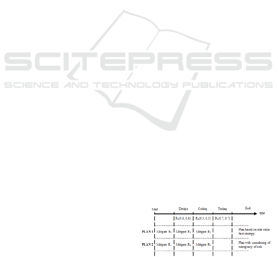
A simple example shown in Figure 1 illustrates
the necessity of considering time elements in risk
mitigation. In Figure 1, R
i
(P
i
, I
i
) represents risk R
i
with probability P
i
and impact I
i
. In this example,
we suppose that: (1) There are three risks which
would occur during design, coding and testing phase
of a hypothetical software development project
respectively. (2) We can only treat one risk at a time
and it takes the same amount of time to mitigate
each risk. (3) The mitigation of each risk eliminates
the risk at the end of the mitigation.
Figure 1: An Example Showing the Necessity of
Managing Time Elements.
PLAN 1 applies the risk value first strategy to
schedule the risk mitigation. Since R
3
has the highest
risk value and R
2
has the lowest risk value, R
3
is
treated first and R
2
is treated at last. Then, R
3
will
365
Zhou P. and K. N. Leung H..
Scheduling Strategies for Risk Mitigation.
DOI: 10.5220/0004409203650376
In Proceedings of the 8th International Joint Conference on Software Technologies (ICSOFT-EA-2013), pages 365-376
ISBN: 978-989-8565-68-6
Copyright
c
2013 SCITEPRESS (Science and Technology Publications, Lda.)
never occur (risk mitigation eliminates R
3
before it
would occur) while R
1
and R
2
would occur during
the time period of their risk mitigation. PLAN 2
considers the emergency of risk that is ignored by
PLAN 1. All risks will be eliminated before they
would occur according to PLAN 2. Thus, it is better
than PLAN 1.
Although the PMI framework and the IEEE
standard point out the necessity of managing time
elements in risk mitigation, there is a lack of
principles and guidelines on how to schedule risk
mitigation with due consideration of time elements.
This paper aims to formally define scheduling
strategy for risk mitigation, identify new scheduling,
and focus on following research questions:
1. Is the traditionally used strategy, risk value first
strategy, a good choice for scheduling risk
mitigation?
2. Is there a best scheduling strategy for most
projects?
3. Is there a worst scheduling strategy for most
projects?
According to (Zhou, 2012), stochastic simulation is
a better choice than other methods to compare the
performance of different scheduling strategies. A
stochastic simulation model (SMRMP) (Zhou and
Leung, 2012) with due consideration of time
elements of risk will be used in our study to obtain
meaningful results.
The paper is organized as follows. We briefly
review the risk management process and the
stochastic simulation model in section 2. In section
3, we formally define scheduling strategy for risk
mitigation, identify new scheduling strategies and
propose a metric to measure the performance of
scheduling strategy. In section 4, we compare the
performance of identified scheduling strategies and
answer the research questions. At last, we conclude
our study and outline the future work in section 5.
2 LITERATURE REVIEW
2.1 Project Risk
Risk is a potential event that would impact the
project. It has two basic attributes, risk probability
(P) and risk impact (I). Accordingly, risk is a
function of P and I (Holton, 2004). We use Risk
Value (RV) to represent the measurement of risk. So
(,)RV f P I (1)
For a given project, the project risk set and its risks
are defined as follows.
Def 1. Given a project Z, it includes a set of
identified n risks at time t, RS(Z, t) =
12
, , ,
n
RR R
.
The size of RS(Z, t), | RS(Z, t)| may change as time
elapses since new risks may be identified and added
into RS(Z, t) and expired risks will be eliminated
from RS(Z, t).
Def 2. For any R
i
∈ RS (Z, t), and 1≤i≤|RS (Z, t)|,
R
i
(P
i
, I
i
) represents risk R
i
with probability P
i
and
impact I
i
.
2.2 Risk Management Process
Risk management aims to identify risks and take
actions to reduce or eliminate their probability
and/or impact so that the project is kept from being
damaged by risks. There are many paradigms,
models and standards to guide the risk management
practice, such as risk management paradigm
developed by Software Engineering Institute
(Williams et al., 1999), PMI framework (PMI,
2008), IEEE Std 1540 (IEEE, 2001), AS NZS 4360
(AS/NZS, 2004) and ISO 31000 (ISO, 2009).
Although these models and standards address the
risk management processes in different manners,
they can be mapped to each other to a large extent.
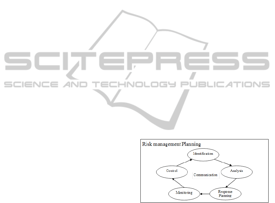
Generally, these paradigms, models and standards
follow the cyclic process shown in Figure 2.
Figure 2: Cyclic Process of Risk Management.
Risk Management Planning defines how to conduct
risk management practices throughout the project. It
is important to provide adequate resources and time
and establish both internal and external context of
risk management.
Risk identification aims to identify risks that
would affect the project objectives and document
their characteristics. Current risk identification
methods include examining the major areas of the
project, collecting information from personnel,
learning from past and applying analytical tools
(PMI, 2008), (Kwan, 2009), (SEI, 2006). Among
these proposed approaches, the taxonomy developed
ICSOFT2013-8thInternationalJointConferenceonSoftwareTechnologies
366

by (Carr et al., 1993) is more popular than others.
The risk analysis aims to understand the
identified risks and provide data to assist in
managing them. Generally, risk analysis includes:
(1) estimate the probability, impact, and the
expected timing of the risk (IEEE, 2001); (2)
analyze risks and prioritize them. Recently, risk
analysis is expanded with the consideration of risk
dependency (Kwan and Leung, 2011).
There are four different options that can be used
to treat a risk. They are avoid, transfer, mitigate and
accept (PMI, 2008), (AS/NZS, 2004). Risk response
planning aims to identifying possible options to
reduce or eliminate risks, assessing these options
and making a plan to implement risk mitigation
activities. To make the best use of resources, a
scheduling strategy is used to determine the risks to
be mitigated and when to mitigate them. The
generally used strategy for scheduling risk
mitigation is “risk value first strategy”.
Risk monitoring and control aims to tracking the
change of all identified risks and identifying new
risks, monitoring residual risks, and evaluating risk
response effectiveness and performance of risk
management (PMI, 2008).
2.3 Time Element in Risk Management
In risk management, time elements exist at both the
project level and risk level. Time elements of risk
management (project-level) are different times that
directly associate with the process of risk
management. Time elements of risk (risk-level) are
different times that directly associate with the risk
from its first identification to its expiration.
All well accepted risk management paradigms,
frameworks and standards clearly define the
lifecycle of risk management. In practice, for each
project, we can clearly define the time duration for
all five risk management processes and the time for
periodical risk review. However, there is no explicit
model for many time elements of individual risk.
“IEEE Standard for Software Life Cycle
Processes - Risk Management” (IEEE, 2001) points
out that practitioners should estimate the expected
timing of the risk and document it. Then,
practitioners need to schedule the treatment of each
risk accordingly. PMI risk management model (PMI,
2008) also points out that the risk mitigation should
be scheduled with due consideration of the expected
occurrence time of the risk. However, both the PMI
framework and the IEEE standard lack principles
and guidelines on how to schedule risk mitigation
with due consideration of many key times of risk.
Consequently, these time elements are rarely used in
practice. This may lead to improper risk mitigation
activities and an ineffective risk management.
Very few studies have explicitly modeled the
time elements of risk. Leung proposed variants of
risk, presented a model of risk lifecycle, and gave
the relationship between the risk variants by explicit
consideration of the occurrence time of risk (Leung,
2010).
Zhou and Leung identified two key time periods
of individual risk for an effective risk management
(Zhou and Leung, 2011). These two time periods are
time period of risk occurrence and risk mitigation.
The time period of occurrence is the duration that a
risk would occur. The time period of mitigation is
the duration for executing planned mitigation
activity of a risk.
Zhou and Leung also proposed a stochastic
simulation model of risk management process with
due consideration of time elements of risks (Zhou
and Leung, 2012). This simulation model can be
used for many risk management issues, such as
understanding of risk management process,
predicting risk management outcome, and making
informed risk management decision. This model will
be presented in next section.
2.4 A Stochastic Simulation Model
Figure 3 shows the “Simulation Model of Risk
Management Process” (SMRMP) proposed in (Zhou
and Leung, 2012).
Conceptual Model
Model Parameters
Yes
Risk Identification
Risk Analysis
Risk Response
Planning
Monitoring and
Control
Risk Management
Planning
Start
Complete?
End of Input
No
strm; etrm;
npr; stpr
m
; etpr
m
stri; etri; nrri
tid
i
p
i
+
; i
i
+
; teo
i
; tlo
i
tms
i
; tmc
i
p
i
-
; i
i
-
nrpr
m
Parameter
Relationships
Assumptions
1. Risk occurrence
2. Risk mitigation
1. Time slicing
2. Null effect of
non-mitigation
factors
3. Non-negative
effect of
mitigation
4. Linear effect of
mitigation
Outputs
occ
i
; toc
i
; imp
i
;
nocc; oimp;
Simulation
Algorithms
Process
Figure 3: Conceptual Model for Risk Management
Process.
Based on a two levels approach, the inputs and
outputs of the model have been identified (Zhou and
SchedulingStrategiesforRiskMitigation
367
Leung, 2012). The first level is the risk level which
focuses on a single risk. The second level is the
project level which considers all risks of the whole
project. Some natural relationships between the
parameters are identified. Algorithms are also
developed to compute output of the simulation from
the input parameters. Besides that, the model has
four assumptions. This model was evaluated to be
valid (Zhou and Leung, 2012) by applying the
paradigm proposed by Sargent (Sargent, 2010).
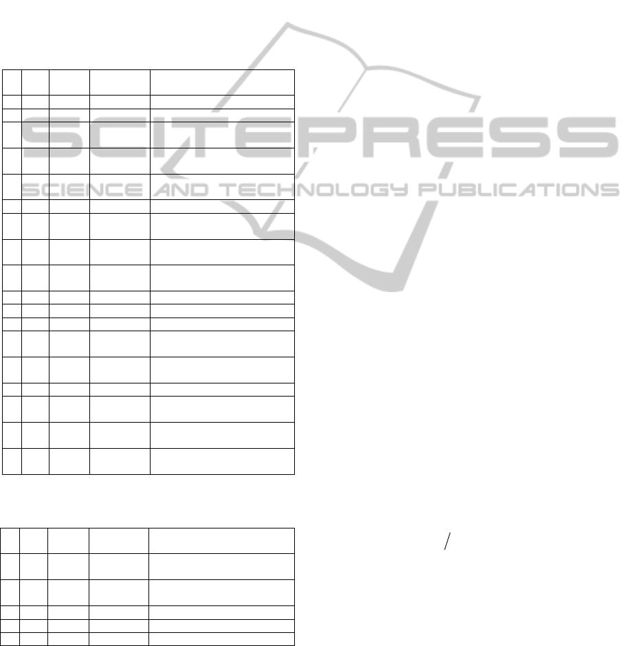
Table 1 and 2 summarize the input parameters
and outputs of SMRMP respectively.
Table 1: Parameters of SMRMP (Zhou and Leung, 2012).
No
Nota
tion
Value Level Description
1
strm
0
*1
project-level start time of risk management
2
etrm
L
*1
project-level end time of risk management
3
stri
>0 project-level
start time of the risk
identification
4
etri
> stri>0 project-level
end time of the risk
identification
5
nrri
≥0 project-level
number of risks identified in
risk identification
6
npr
>0 project-level number of periodical reviews
7
stpr
m
>0 project-level
start time of the m
th
periodical
review
8
etpr
m
>stpr
m
project-level
end time of the m
th
periodical
review
9
nrpr
m
≥0 project-level
number of risks identified in
the m
th
periodical review
10
tid
i
>0 risk-level the time that R
i
is identified
11
teo
i
>0 risk-level earliest time of occurrence of R
i
12
tlo
i
>teo
i
>0 risk-level latest time of occurrence of R
i
13
p
i
+
∈ (0, 1)
risk-level
probability of R
i
when it is first
identified
14
i
i
+
∈ (0, 1]
risk-level
impact of R
i
when it is first
identified
15
tms
i
≥ tid
i
>0 risk-level mitigation start time of R
i
16
tmc
i
∈ ( tms
i
,
tlo
i
]
risk-level mitigation close time of R
i
17
p
i
-
∈ [0, 1)
risk-level
expected probability of R
i
after
the mitigation
18
i
i
-
∈ [0,1]
risk-level
expected impact of R
i
after the
mitigation
*1 suppose the risk management starts at time 0 and ends at time L
Table 2: Outputs of SMRMP (Zhou and Leung, 2012).
No Nota
tion
Value Level Description
1
occ
i
Yes/No risk-level represent whether R
i
occurs or
not
2
toc
i
∈ (teo
i
,
tlo
i
]
risk-level occurrence time of R
i
if it
occurs
3
imp
i
>0 risk-level impact of R
i
if it occurs at toc
i
4
nocc
≥0 project-level number of all occurred risks
5
oimp
≥0 project-level overall impact of all risks
The model assumptions are listed as follows.
1. Time slicing. For a given project Z, the time
period of its risk management is equally divided
into L time intervals with a set of L+1 time
points,
() {0,1,2,...,}TP Z L
. All management
activities start at one of these time points and
take integral multiple of intervals.
2. Null effect of non-mitigation factors. The factors
not related to risk mitigation, such as change of
external and internal risk management
environments, will not change the probability
and impact of a risk.
3. Non-negative effect of mitigation. Risk
mitigation will not increase the probability and
impact of a risk. It is reasonable since risk
mitigation should not increase the risk and is
often effective in reducing the risk.
4. Linear effect of mitigation. The probability and
impact of a risk will linearly decrease during its
mitigation period from p
i
+
to p
i
-
and from i
i
+
to i
i
-
respectively.
Model users should go through the whole process of
risk management to determine the values of model
parameters based on the parameter relationships and
model assumptions. After inputting all model
parameters, users can run the simulation for each
risk, and get outputs which can help to predict the
expected impact on projects.
Since the probability and impact of a risk may
change with time, EOR and EAI are introduced to
measure the expected occurrence rate and expected
impact during (teo
i
, tlo
i
] (Zhou and Leung, 2012).
Since a risk cannot be repeated in real-life projects,
IIR is introduced to facilitate the computation of
EOR and EAI (Zhou and Leung, 2012).
Def 3. Independent and Identical Risks (IIR): If R
1
and R
2
are independent risks and have the
exactly same values in all risk-level
parameters, then they are independent and
identical risks (IIR).
Def 4. Suppose there are N IIRs, if M risks occurred
among all N risks when N is sufficiently
large, then EOR=M/N.
Def 5. Expected Actual Impact (EAI): Suppose there
are N IIRs, if M risks occurred among all N
risks when N is sufficiently large, then
EAI=
i
M
imp N
, where
i
M
imp
is the total
impact of M occurred risks.
3 SCHEDULING STRATEGY
FOR RISK MITIGATION
3.1 Definition of Scheduling Strategy
To facilitate the definition of scheduling strategy for
ICSOFT2013-8thInternationalJointConferenceonSoftwareTechnologies
368

risk mitigation, we first define the set of risks need
to be treated at time t and the resource assigned for
risk mitigation.
Def 6. Given a risk set TRS(Z, t) and TRS(Z, t)⊆
RS(Z, t), ∀R
j
∈ TRS(Z, t), R
j
is a risk which
does not have a mitigation plan and waiting
for treatment, and ∀R
k
∈ RS(Z, t)- TRS(Z, t),
R
k
is a risk which is acceptable and need not
to be treated or has been scheduled for
mitigation.
We abstract the human resource for risk mitigation
as a set of processors which have different
capabilities to mitigate risk.
Def 7. For a given project Z, a set of k processors at
time t, ProS(Z, t) =
{|0}
i
processor i k
,
are available for risk mitigation.
∀processor
i
∈ ProS(Z,t), CAP(processor
i
)=c
i
,
where CAP(processor
i
) is the capability of
processor
i
for risk treatment and c
i
is a real
number greater than 0.
The capability of a processor can be considered as 1
if it represents the capability of a team member that
has normal capability for risk mitigation. Then the
capabilities of all processors can be estimated
according to capabilities of different team members.
For R
i
assigned to processor
j
(0<j≤k),
ii ij
tmc tms Effort c
(2)
where Effort
i
is the estimated effort for the treatment
of R
i
.
Note that the processor is assumed to process one
risk at a time. However, it is possible that a team
member may treat two (or more) different risks at
the same time in practice. In this case, this team
member can be abstracted as two (or more)
processors with capability equal to the capability of
the team member. From this point of view, we can
consider each processor can process one risk at a
time.
For convenient sake, in this study, we assume all
processors in ProS(Z, t) have the same capability
equal to 1, and each processor processes one risk at a
time. Then the effort of mitigating a risk can be
estimated according to the capability of the
processor and the time needed to mitigate the risk.
Note that the time unit should be consistent with the
time unit adopted in the simulation model.
The mitigation scheduling of a project Z aims to
allocate a set of m risks (|TRS(Z, t)|=m) to a set of k
processors (|ProS(Z, t)|=k), to minimize the expected
impact on Z. Suppose there is only one processor
(k=1), then there are m! different sequences to
allocate risks to this single processor. We can choose
the schedule with the minimal expected impact
among all m! different sequences. However, this
approach is unreasonable in practice because the
time for finding the best option from m! options is
non-polynomial. The situation become more
complicated when there are more processors (k>1).
Thus there is a need to develop scheduling strategies
to determine the sequence for treating the risks in
TRS(Z, t).
Based on TRS(Z, t) and ProS(Z, t), we define
scheduling strategy for risk mitigation as follows.
Def 8. Scheduling strategy for risk mitigation is an
algorithm that takes TRS(Z, t) and ProS(Z, t)
as input and generates a scheduled risk
mitigation plan as its output. For each R
i
∈
TRS(Z, t), it decides whether R
i
is to be
mitigated, and then chooses processor
j
∈
ProS(Z, t) to mitigate R
i
during a selected
time period.
Since risk mitigation aims to prevent the project
from impacted by the risks, the performance of a
scheduling strategy S can be measured by the
expected impact of all risks in TRS(Z, t),
EAI(S|TRS(Z,t)), after S has been applied to TRS(Z,
t). EAI(S|TRS(Z,t)) is defined as
Def 9. Let EAI(S|TRS(Z,t)) be the expected impact
of all risks in TRS(Z, t) after a scheduling
strategy S has been applied to TRS(Z, t).
(,)
|(,) ()
i
i
RTRSZt
EAI S TRS Z t EAI R
(3)
where EAI(R
i
) is EAI of R
i
. EAI(S|TRS(Z,t)) ranges
in (0, | TRS(
Z, t)|) because EAI ranges in (0, 1).
A higher value of EAI(S|TRS(Z,t)) means a
higher expected impact on the project and indicates
a lower performance of
S. Thus we define the
performance of a scheduling strategy as follows.
Def10. Let Perf(S) represents the performance of a
scheduling strategy
S applied to the risk set
TRS(
Z, t). For two scheduling strategies S
i
and
S
j
,
Perf(S
i
)>Perf(S
j
) when EAI(S
i
|TRS(Z,t))<EAI(S
j
|TRS(Z,t));
Perf(S
i
)=Perf(S
j
) when EAI(S
i
|TRS(Z,t))=EAI(S
j
|TRS(Z,t));
Perf(S
i
)<Perf(S
j
) when EAI(S
i
|TRS(Z,t))>EAI(S
j
|TRS(Z,t)).
3.2 New Scheduling Strategies
Traditionally, risk value first strategy (V strategy) is
used in practice. However, it does not consider the
time elements of risk. Besides the V strategy, we
propose several new strategies.
1.
Emergency first strategy (E strategy).
SchedulingStrategiesforRiskMitigation
369

Emergency first strategy first orders all risks
according to their T
eo
, then risks with an earlier T
eo
will be treated earlier. For example, suppose teo
i
=30
and teo
j
=50 are earliest occurrence time of R
i
and R
j
respectively, then R
i
will be mitigated first.
The principle behind this strategy is that we
should mitigate the risk before it would occur. The
best case of applying this strategy is all risks are
mitigated before they would occur. No risk will
occur if all mitigations are successful in eliminating
the risks. The example shown in Figure 1 is a good
example of applying this strategy.
2.
Lowest effort first strategy (L strategy).
Lowest effort first strategy first orders all risks
according to the efforts needed for mitigating the
risk, then risks requiring a lower effort will be
treated earlier. For example, suppose 40 Man-hour
and 80 Man-hour are needed effort to mitigate R
i
and R
j
respectively, then R
i
will be mitigated first.
The principle behind this strategy is that we can
mitigate more risks within the same time period
because mitigating a risk with lower effort will use
less time. Consequently, we may prevent more risks
from occurring and this leads to a low overall impact
of the project.
3.
Combined strategies.
We consider applying combination of V, E and L
strategies at the same time by constructing some
combined strategies. For example, we can combine
the risk value first strategy and emergency first
strategy together. The resulting strategy first
prioritizes all risks based on their risk value and T
eo
respectively, producing two risk lists. For risk R
i
, a
score is calculated by combining its priority values
from these two risk lists. Using the calculated
scores, all risks can be finally prioritized and then
scheduled so that a risk with a higher priority will be
treated earlier.
As there are three basic strategies, V strategy, E
strategy and L strategy, we can create four combined
strategies, VE strategy (combined V with E), VL
strategy (combined V with L), EL strategy
(combined E with L) and VEL strategy (combined
all three basic strategies). We assign weights, w
1
, w
2
and w
3
, to the priority according to the three basic
strategies. In this study, we apply equal weights to
these three strategies as there are no prior studies
showing that one basic strategy is better than
another. The combined strategy is equivalent to VE
Strategy when w
1
= w
2
and w
3
=0, VL Strategy when
w
1
= w
3
and w
2
=0, EL Strategy when w
2
= w
3
and
w
1
=0 and VEL Strategy when w
1
= w
2
= w
3
. We can
create more combined strategies by using unequal
weights in the future.
Table 3 shows examples of applying different
strategies to schedule risk mitigation. The number
shown under basic strategies is the priority that the
risk is scheduled (a lower value indicates a higher
priority). For example, R
1
is scheduled first, and
then followed by R
2
, R
3
and R
4
when applying V
strategy. The score value under combined strategies
is calculated by adding the priority of corresponding
basic strategies. For example, for VE strategy, the
score of the 5
th
column is the result of adding the
priority in V strategy (the 2
nd
column) and that in E
strategy (the 3
rd
column). Then all risks are
prioritized based on their scores. Note that if two or
more risks have the same score, then they can be
prioritized in any order. Since we have to choose
one order to mitigate the risks, in our study, the risk
with a smaller index will get a higher priority when
several risks have the same score. For example, R
2
and R
3
have the same score of 4 under VL strategy.
Then R
2
is assigned a higher priority than R
3
and
will be mitigated earlier than R
3
.
Table 3: Examples of Mitigation Strategies.
Risk
Basic Strategy Combined Strategy
V E L VE VL EL VEL
Pri Pri Pri Sco Pri Sco Pri Sco Pri Sco Pri
R
1
1 2 4 3 1 5 3 6 3 7 2
R
2
2 3 2 5 3 4 1 5 2 7 3
R
3
3 1 1 4 2 4 2 2 1 5 1
R
4
4 4 3 8 4 7 4 7 4 11 4
We next formally define above scheduling
strategies. Suppose
12
( , ) , , ......,
N
TRS Z t R R R
. Let
Rank(R
i
|RL) be the rank of R
i
in the prioritized risk
list (RL) of n risks, with rank of 1 indicating the first
risk of RL and rank of n indicating the last risk of
RL. That is a lower rank value indicates a higher
priority.
Recall that RV
i
, teo
i
and Effort
i
(1≤i≤N) represent
the risk value, earliest time of occurrence and
estimated mitigation effort of R
i
respectively.
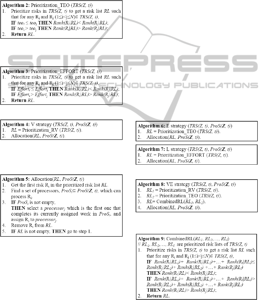
Algorithm 1, 2 and 3 shows three different ways to
prioritize TRS(Z, t).
Algorithm 1 produces a risk list such that a risk with
a higher risk value will have a higher priority.
As mentioned earlier, two risks with the same score
will be prioritized according to their risk indexes.
ICSOFT2013-8thInternationalJointConferenceonSoftwareTechnologies
370
Thus, in Algorithm 1, R
i
has a higher priority than R
j
when RV
i
= RV
j
and 1≤i<j≤N. Similarly, in
Algorithm 2, 3, and 9, if two risks have the same T
eo
,
estimated mitigation effort, and computed score
respectively, then they will be prioritized according
to their risk indexes too.
Algorithm 2 produces a risk list such that a risk with
an earlier T
eo
will have a higher priority.
Algorithm 3 produces a risk list such that a risk with
a smaller mitigation effort will have a higher
priority.
V strategy is defined as Algorithm 4.
Allocation(RL, ProS(
Z, t)) is shown as Algorithm 5,
which allocates the prioritized risks to the processors
in ProS(
Z, t) such that the risk with a higher priority
will be allocated first.
Note that a processor is not able to process risk R
i
if
it cannot complete the mitigation of R
i
before its
latest time of occurrence. For example, suppose a
processor completes its currently assigned work at
t=50. If tlo
i
=40, then the processor is not able to
process R
i
since the mitigation after the latest time
of occurrence does not make sense. Another
example is that suppose tlo
i
=60 and the time length
for mitigating R
i
is 20. In this case, if the mitigation
is started at t=50, the processor cannot complete the
mitigation before tlo
i
(actually it completes the
mitigation at t=50+20=70).
There may exist more than one processor that
can process risk R
i
at the same time. Then, we
should select the first processor that completes its
work because the risk in RL should be treated as
early as possible. For example, assume some risks
have been assigned to processor
1
and processor
2
,
processor
1
will complete its currently assigned
works at t=20 and processor
2
will complete its
currently assigned works at t=40. Suppose teo
i
, tlo
i
and Effort
i
are 40, 60 and 10 respectively. Then,
both processor
1
and processor
2
can process R
i
because they can complete the mitigation of R
i
(at
t=30 and t=50 respectively) before tlo
i
=60. In this
case, we should select processor
1
to mitigate R
i
because it completes its currently assigned work
earlier (at t=20) and consequently the mitigation of
R
i
can be started earlier if it is assigned to
processor
1
.
Also, there may not exist any processors that can
process risk R
i
if they are all busy. In this case, R
i
is
removed from RL directly.
E strategy and L strategy are defined as Algorithm 6
and 7 respectively.
Algorithm 8 defines VE strategy.
CombinedRL(RL
1
, RL
2
,…, RL
l
) is shown as
Algorithm 9, which produces a risk list such that the
SchedulingStrategiesforRiskMitigation
371

risk with a lower score (which is computed by its
rank from input risk lists, RL
1
, RL
2
,…, RL
l
) will have
a higher priority.
VL, EL and VEL strategies can be implemented
similarly to Algorithm 8.
4 PERFORMANCE
OF SCHEDULING
STRATEGIES
Next, we compare the performance of different
strategies by running simulations based on SMRMP.
Let imp(R) denotes the impact of a given risk R in
one simulation.
1
()/
N
i
i
imp R N
is the average
impact of R in N simulations, where imp(R)
i
is the
impact of R in the i
th
simulation (1<i≤N). According
to (Zhou and Leung, 2012), if N is sufficiently large,
then
1
()/
N
i
i
imp R N
follows a normal distribution
with mean EAI(R). That is
1
()/
N
i
i
imp R N
can be
used to approximate EAI(R) when N is sufficiently
large. Let imp(
S|TRS(Z,t)) denotes the total impact
of all risks of TRS(
Z,t) in one simulation with
strategy
S. Then,
1
(| (,))/
N
i
i
imp S TRS Z t N
can
be used to approximate EAI(S|TRS(Z,t)) when N is
sufficiently large. imp(
S|TRS(Z,t))
i
is the total
impact of all risks of TRS(
Z,t) in the i
th
simulation
(1<i≤N). For example, after applying V strategy to
TRS(
Z,t) and running simulation for 1000 times, the
average imp(V|TRS(
Z,t)) from these simulations can
be used to measure the performance of V strategy.
Def11. Let average overall impact, AVEOI(S)
denotes the average imp(
S|TRS(Z,t)) of
running a large number (N) of simulations on
TRS(
Z,t) with strategy S. AVEOI(S) is
computed as
1
() ( | (,))
N
i
i
A
VEOI S imp S TRS Z t N
(4)
If all risks of project Z need to be scheduled for
mitigation, then imp(
S|TRS(Z,t)) can be replaced by
oimp of SMRMP because oimp is the total impact of
the project.
Since AVEOI(
S) is an approximation of
EAI(S|TRS(Z,t)), it can be used to measure the
performance of
S. That is a lower AVEOI(S)
indicates
S has a higher performance and a higher
AVEOI(
S) indicates S has a lower performance.
We are also interested in the difference in
performance of two strategies when they are applied
to the same project.
Def12. Suppose S
i
and S
j
are two scheduling
strategies that are applied to project
Z, with
AVEOI(
S
i
) ≥ AVEOI(S
j
). PIP (Percentage of
Improved Performance) is defined as
,( () ()) ()
ij i j i
PIP S S AVEOI S AVEOI S AVEOI S
(5)
PIP(S
i
,S
j
) measures the relative improvement of
impact of
S
j
over that of S
i
. PIP(S
i
,S
j
) ranges in [0,
1]. PIP(S
i
,S
j
) equals 0 when AVEOI(S
i
) =
AVEOI(
S
j
), indicating that S
i
and S
j
have the same
performance. It equals 1 when AVEOI(
S
j
) = 0. The
higher the value of PIP(S
i
,S
j
), the larger the
improvement of
S
j
over S
i
.
4.1 Cases for Simulation
In this section, we identify the cases used for
comparing performance of different scheduling
strategies. Risk mitigation can be viewed as using a
set of processors to mitigate a given set of risks. The
processor takes risks as input and mitigates them.
So, the risk set is the input to the risk mitigation. For
output, we are most interested in the effectiveness of
risk mitigation. Next, we identify different cases
from these two aspects of input and output of risk
mitigation.
The input to risk mitigation is a set of risks
TRS(
Z, t). The external context of these risks is a
project
Z of a certain project type (Cadle and Yeates,
2008), size and application domain. The basic
internal attributes of risk are probability and impact.
First, we explore the external context and internal
attributes of risk to identify key parameters for
simulation.
After identifying the response option of
mitigating a risk, the next issue is to determine when
and which processor should work on mitigating the
risk. Thus, the scheduling problem can be
formulated as how to order the mitigation of a set of
risks given a set of processors. Consequently, the
type of project, (i.e. software development project,
system enhancement project and so on), and the
domain of the project (i.e. banking, medical,
telecommunication and so on) are not important in
the context of our study.
A large project having a large number of risks
and a large mitigation team is similar with a small
project having a small number of risks and a small
mitigation team when scheduling risk mitigation.
For example, suppose a large project has 100 risks
and 100 processors, and another project have 20
ICSOFT2013-8thInternationalJointConferenceonSoftwareTechnologies
372

risks and 20 processors. In both cases, each risk can
be allocated to a unique processor and all risks can
be treated at the same time. Therefore, compared
with the ratio of the number of risks to the number
of processors, the project size is less important for
scheduling risk mitigation because it may indicate
the number of risks only and cannot represent the
size of mitigation team.
Def13. RRP (Ratio of Risks to Processors) is
defined as
(,) (,)RRP TRS Z t ProS Z t
(6)
where TRS(
Z, t) and ProS(Z, t) are the set of risks
waiting for mitigation and the set of processors
respectively.
RRP is more meaningful than the number of
risks for scheduling risk mitigation because it
integrates both the number of risks and number of
processors. RRP is a better parameter for the
simulation when compared to the number of risks.
It is meaningful that we use different RRP values
obtained from different contexts to represent
different cases. We obtain RRP values from
different combinations of project sizes and
mitigation team (processor) sizes. We assume the
number of risks is related to the project size so that
larger projects will have more risks. In this study, we
consider two categories of project size, large project
and small project, and consider three categories of
team size, large team, medium team and small team.
We will consider more categories of project size and
team size in future study. Note that we will not
consider following two combinations: (1) small
project and a large mitigation team, leading to a very
small RRP and (2) large project and a small
mitigation team, leading to a very large RRP,
because effective risk mitigation is hard to be
achieved in this case. Thus we consider four most
common cases: 1. small project (with a small
number of risks) and a small mitigation team, 2.
small project and a medium mitigation team, 3. large
project (with a large number of risks) and a medium
mitigation team and 4. large project and a large
mitigation team. We choose following values for
RRP for the simulations.
1.
| TRS(Z, t)|=20, | ProS(Z, t)|=2, with RRP=10
2.
| TRS(Z, t)|=20, | ProS(Z, t)|=4 with RRP=5
3.
| TRS(Z, t)|=60, | ProS(Z, t)|=4, with RRP=15
4.
| TRS(Z, t)|=60, | ProS(Z, t)|=15, with RRP=4
Larger projects usually require a longer development
lifecycle. So, projects of different sizes would have
different time periods of risk management.
However, the time unit used in SMRMP is a relative
time scale. Hence, different time periods can be
normalized into 100 time units. Consequently, we
can consider that
strm =0 and etrm =100.
For the internal attributes of risk, we consider the
distribution (DoP) of the probability and the
distribution (DoI) of impact of risks. To be
meaningful, we consider four different distributions
which represent majority of risks having large RV,
medium RV, small RV and randomly distributed RV
respectively.
(1) Both P and I follow the distribution shown in
Figure 4-I. It implies that most risks have medium P
and I. (2) Both P and I follow the distribution shown
in Figure 4-II. It implies that most risks have high P
and I. (3) Both P and I follow the distribution shown
in Figure 4-III. It implies that most risks have low P
and I. (4) Both P and I follow the distribution shown
in Figure 4-IV.
Figure 4: Different Distributions of P and I.
Note that the distribution of probability and the
distribution of impact need not be the same. In our
study, the probability and impact of a risk are
independent even if they follow the same
distribution. In future study, we will consider more
cases with different distributions of probability and
distributions of impact. The other attributes of risk,
such as the time period of occurrence and efforts to
mitigate a risk are randomly generated (details will
be provided in section 4.2).
To model the effectiveness of risk mitigation, we
consider two cases: (1) Full reduction. Each
processor can eliminate the assigned risks. (2)
Random reduction. Each processor randomly
reduces the probability and impact of assigned risks.
That is each processor reduces the probability and
impact of R
i
from p
i
+
and i
i
+
to p
i
-
=r
1
×p
i
+
and i
i
-
=r
2
×i
i
+
respectively, where r
1
and r
2
are random
numbers in [0, 1].
Note that we will not consider the case of Zero
reduction that a processor does not reduce the
probability and impact of assigned risks because this
case is same as no mitigation. Naturally all
scheduling strategies give the same performance for
this case.
In summary, with due consideration of different
inputs (external context and internal attributes of
TRS(
Z, t)), and outputs (effectiveness of mitigation)
SchedulingStrategiesforRiskMitigation
373

of processor, we obtain totally 4×4×2=32 different
cases.
4.2 Parameters of SMRMP
To simulate different cases, we first identify the
values of parameters of SMRMP. Based on settings
discussed in last section, we select values or
probability distributions for the parameters of
SMRMP (see Table 1). For each case, we set the
parameters of SMRMP as follows.
1.
Parameters of SMRMP at project-level.
(1)
strm =0 and etrm =100. (2) we consider that all
risks are identified in the first risk identification and
no new risks are identified in periodical reviews.
The reason is in comparing performance of different
scheduling strategies, it is not important to consider
the effect of the periodical reviews, since we can
apply scheduling strategies to the risk set TRS(
Z, t)
at any time. At the beginning of the project, we can
select a scheduling strategy based on risks identified
in risk identification to generate a schedule for risk
mitigation. Then we can repeat the strategy selection
at the end of each periodical review if new risks
have been identified. Consequently, we just assume
all risks are identified at the beginning of risk
management. For convenient sake, we set the start
time of risk identification to 0 (
stri=0) and the end
time of risk identification to 1(
etri=1) respectively.
2.
Parameters of SMRMP at risk-level.
(1)
tid
i
of any risk R
i
is 1 since etri=1. (2) p
i
+
and i
i
+
of risk R
i
are generated according to the distribution
of the case. (3)
p
i
-
and i
i
-
of risk R
i
are generated
according to mitigation effectiveness of the case. (4)
the time period of occurrence of all risks is randomly
generated within the lifecycle of risk management,
because risks can occur at any phase of the project.
Suppose we identify risk R
i
before it would occur,
then [
teo
i
, tlo
i
] should be in the range [1, 100] since
tid
i
=1 and etrm =100. (5) the effort of mitigating a
risk is randomly generated within the available time
for its mitigation. Since the effort for mitigating a
randomly generated risk is unpredictable, we
consider that a randomly generated mitigation effort
is a good choice. According to the effort, the
scheduling strategy is applied to determine whether
R
i
can be mitigated by a specific processor and the
time to mitigate it. Thus, the time period of risk
mitigation will be determined according to the
selected scheduling strategy.
4.3 Results of Simulation
We generate 1000 projects for each case and apply
all 7 scheduling strategies to each project. Therefore
there are 7000 combinations of projects and
scheduling strategies for each case. We run 1000
simulations for each combination to compare the
performance of different scheduling strategies.
We run simulations on all 32 cases. Table 4
summarizes the chance of different strategies to be
the best/worst strategy among 32 cases. For
example, the chance for V strategy to be the best
strategy in 32 different cases ranges in [0.1%, 66%].
V strategy has 21% chance to be the best strategy on
average (that is, it is the best strategy for 21% of all
32000 sample projects).
Table 4: Summary of Strategies to be the Best/Worst.
(%)
V E L VE VL EL VEL
chance to be
the best
Range 0.1-66 0-5 0-17 0.3-36 4-65 0-13 2-34
Ave 21 0.8 4 14 32 4 24
cases to be the best 8 0 0 3 18 0 3
chance to be
the worst
Range 0-17 45-99 0-45 0-14 0-16 0-4 0-43
Ave 5 68 15 4 1 6 0.8
cases to be the
worst
0 32 0 0 0 0 0
Table 5 shows average AVEOI of 7 identified
strategies from all 32 cases. From Table 5, we find
that Perf(VL)> Perf(VEL)> Perf(V)> Perf(VE)>
Perf(L)> Perf(EL)> Perf(E) for all sample projects.
Table 5: Average AVEOI of All Cases.
V E L VE VL EL VEL
AVEOI 5.8815 7.0276 6.1485 5.9916 5.5475 6.1607 5.6132
Table 6 shows the average PIP between the best
strategy and the worst strategy and other 7 identified
strategies. From Table 6, we find that: On average,
always applying the best strategy can improve the
performance by 10% over the traditional V strategy,
by 31% over the worst strategy, and by at least 8%
over other strategies.
Table 6: Average AVEOI of All Cases.
B-W B-V B-E B-L B-VE B-VL B-EL B-VEL
0.31 0.10 0.28 0.19 0.13 0.08 0.19 0.09
4.4 Answers to the Research Questions
Next we answer the research questions listed at the
beginning of the paper.
1.
Is the traditionally used strategy, risk value first
strategy (V), a good choice for scheduling risk
mitigation?
From the Table 4, we find that V strategy is the best
strategy for only 21% of all 32000 sample projects,
and has a lower chance to be the best strategy than
ICSOFT2013-8thInternationalJointConferenceonSoftwareTechnologies
374

VL and VEL strategy. It also has a higher chance to
be the worst strategy than three other strategies (VE,
VL and VEL). From Table 6, we find that the best
strategy can improve the performance by 10% over
V strategy on average. That is, applying the best
strategy for each project will improve the
performance of always applying the V strategy by
10%. Moreover, V strategy has a lower performance
than VL and VEL strategy on average. Thus, V
strategy is not a good choice for scheduling risk
mitigation.
2.
Is there a best scheduling strategy for most
projects?
From simulation results, we find that none of the 7
strategies can be a “dominate strategy” for projects
of a certain case. The dominate strategy of a case is
the strategy that is the best strategy for most projects
(i.e. more than 70% projects) of the case. From
Table 4, we find that VL strategy has the highest
chance to be the best strategy for all sample projects
and in 18 cases out of 32 cases. It is the best strategy
for 32% projects of all 32000 sample projects. It has
only 1% chance to be the worst strategy. This
performance is similar to that of VEL strategy
(0.8%) and is lower than that of the other 5
strategies. However, VL strategy is the best strategy
for less than half of projects (only 32% projects)
from all cases. In summary, there is no strategy that
can be the best strategy for most projects of all cases
or for most projects of a certain case.
3.
Is there a worst scheduling strategy for most
projects?
From Table 4, we find that E strategy has the highest
chance to be the worst strategy in all 32 cases. It has
at least 45% chance and 68% chance on average to
be the worst strategy for all cases. Moreover, it has a
lower performance than all other strategies. So, it is
the least preferred strategy for scheduling risk
mitigation. However, it can be the best strategy for
some projects. Among 32000 sample projects, it is
the best strategy for 0.8% projects.
5 CONCLUSIONS
In this paper, we formally define the scheduling
strategy for risk mitigation, identify some new
scheduling strategies with due consideration of key
time elements if risk, and compare their performance
by applying a stochastic simulation model.
From the simulation results, we find that, for all
tested cases: (1) The traditionally strategy, V
strategy, is not a good choice for scheduling risk
mitigation. The best strategy can improve the
performance of V strategy by 10% on average. That
means we should not always use V strategy. (2)
There is no strategy that can be the best strategy for
most projects or for most projects of a certain case.
This indicates we should not always apply the same
strategy to all projects or to the projects of a certain
case. (3) For scheduling risk mitigation, E Strategy
is the least preferred strategy among 7 identified
strategies. According to above findings, we do not
recommend the user to always apply the same
strategy to all projects. We suggest the user find the
best strategy for each project by running simulation.
Our study has some limitations: (1) The “Null
effect of non-mitigation factors” assumption and
“Linear effect of mitigation” assumption are a bit
strong for real projects. (2) Compared to the variety
of real-life projects, we only run simulation for 32
different cases covering a total of 32000 projects.
In the future, we shall: (1) Expand our study by
running more simulation with due consideration of
effects of non-mitigation factors. (2) Expand our
study with some non-linear risk reduction models,
such as polynomial models. (3) Identify new
mitigation scheduling strategies. In the future, we
will try to identify better strategies. (4) Apply the
proposed methods to real-life projects including
some large-scale applications to confirm its value.
ACKNOWLEDGEMENTS
This research is partly supported by Hong Kong
Polytechnic University grant G-YK27.
REFERENCES
AS/NZS 2004. AS/NZS 4360: Risk Management.
Standards Australia International Ltd.
Boehm, B. W. 1989. Software Risk management, IEEE
Computer Society Press.
Cadle, J. & Yeates, D. 2008. Project Management for
Information Systems,
Harlow, England, Prentice Hall.
Carr, M. J., Konda, S. L., MONARCH, I., ULRICH, C. &
WALKER, C. F. 1993. Taxonomy-based risk
identification. Pittsburgh, PA: Software Engineering
Institute.
Heemstra, F. J. & Kusters, R. J. 1996. Dealing with Risk:
A Practical Approach.
Journal of Information
Technology,
11, 333-346.
Holton, G. A. 2004. Defining Risk.
Financial Analysts
Journal,
60, 12-25.
IEEE 2001. IEEE Std 1540-2001: IEEE Standard for
Software Life Cycle Processes—Risk Management.
SchedulingStrategiesforRiskMitigation
375

New York: IEEE SA.
ISO 2009. ISO 31000: Risk Management - Principle and
Guidelines. Switzerland: International Standard
Organization.
Keil, M., Cule, P. E., Lyytinen, K. & Schmidt, R. C. 1998.
A Framework for Identifying Software Project Risks.
Communications of ACM.
Kwan, T. W. 2009. A Risk Management Methodology with
Risk Dependencies.
Doctor of Philosophy, The Hong
Kong Polytechnic University.
Kwan, T. W. & Leung, H. K. N. 2011. A Risk
Management Methodology for Project Risk
Dependencies.
IEEE Transactions on Software
Engineering,
37, 635-648.
Leung, H. K. N. 2010. Variants of Risk and Opportunity.
17th Asia Pacific Software Engineering Conference.
Lister, T. 1997. Risk Management is Project Management
for Adults.
IEEE Software.
PMI 2008. A Guide to the Project Management Body of
Knowledge,
Newtown, PA, Project management
Institute.
Sargent, R. G. 2010. Verification and Validation of
Simulation Models.
Proceedings of the 2010 Winter
Simulation Conference.
SEI 2006. CMMI® for Development Version 1.2,
Pittsburgh, PA, Software Engineering Institute.
Sherer, S. A. 2004. Managing Risk Beyond the Control of
IS Managers: The Role of Business Management.
Proceedings of 37th Hawaii International Conference
on System Sciences.
Hawaii.
Williams, R. C., Pandelios, G. J. & Behrens, S. G. 1999.
Software Risk Evaluation (SRE) Method Description
(version 2.0). Pittsburgh, PA: Software Engineering
Institute.
Zhou, P. 2012.
Managing Time Elements of Risk. Doctor
of Philosophy, The Hong Kong Polytechnic
University.
Zhou, P. & Leung, H. K. N. 2011. Improving Risk
Management with Modeling Time Element.
15th
IASTED International Conference on Software
Engineering and Applications.
Dallas, USA.
Zhou, P. & Leung, H. K. N. 2012. A stochastic simulation
model for risk management process.
19th Asia-Pacific
Software Engineering Conference (APSEC 2012).
Hong Kong.
ICSOFT2013-8thInternationalJointConferenceonSoftwareTechnologies
376
