
Technology Migration Determination Model for DRAM Industry
Ying-Mei Tu and Chao-I Wang
Department of Industrial Management, Chung Hua University, 300, HsinChu City, Taiwan
Keywords: Technology Migration, Dram, Technology Roadmap, Learning Curve.
Abstract: Due to short life cycle of DRAM industry over the past decade, the product generation and technology
migration have to be quickly enhanced. When technology migration occurred, DRAM companies always
used the past experiences to proceed with process changes. However, the issues are totally different
particularly in the best practice of technology migration that caused the companies suffered many
uncertainties. In this work, a model to determine the timing of technology migration is proposed. The model
is based on technology roadmap to set the timing of migration under maximum profit condition. A stable
growth trend is assumed for market demand to decide the revenue. Furthermore, the time-cost function of
new generational equipment and the theory of learning curve are introduced as the factors to determine the
manufacturing cost and profit. Consequentially, the best timing is determined with maximum profit.
1 INTRODUCTION
DRAM industry is a capital intensive, high-tech
industry with complex processes and technology
migration for DRAM manufacturers has been a very
challenging aspect and more time consuming. Since
there is no any physical capacity expansion over the
past 5 years in Taiwan, all DRAM manufacturers
were relying more than ever on technology
migration to increase supply and reduce cost.
Furthermore, product generation and technology had
been quickly enhanced due to short product life
cycle. When new technology emerges, it reveals that
a lower cost and more effective operation model
emerged (Cainarca, 1989). Simultaneously, it also
means the current competitive advantages of the
company will be jeopardized (Hastings, 1994).
Under this circumstance, manufactures have to
launch new technology and retrofit generational
equipment to meet the market demand and reduce
manufacturing cost. Chou et al., (2007) pointed out
the technology life cycle of semiconductor
manufacturing usually won’t be over three years and
the time of technology generational transition should
take about nine months. Therefore, the
semiconductor manufacturers always face the
dilemma between capacity expansion and new
technology migration. Generally, the major
competition factor of DRAM industry is the
manufacturing cost. That is why the frequency of
technology migration is higher than foundries.
There are many researches regarding to the
influence of new technology introducing. Chand
and Sethi based on the enhancement of process
stability by the new generational equipment to plan
the replacement of new generation capacity.
However, the impacts on the other factors and the
lead time of replacement were not taken into account.
Cohen and Halperin proposed a method to determine
the timing of technology migration which was based
on the price changes of new equipment as well as its
impact on the cost to find the best timing for
migration. Rajagopalan et al. combined the above
two studies and proposed a capacity planning model
under the impact of technology evolution. The linear
programming was applied and the concept of
timeline was added to the decision of capacity
expansion or replacement decisions. Pak et al.,
(2004) proposed a methodology of capacity planning
which focused on the capacity shortage to plan the
capacity requirement and the influence from cost of
new technology capacity was taken into account.
Furthermore, the sensitivity analysis was applied to
determine how sensitive of this plan in the changes
of market demand. Chien and Zheng, (2002)
proposed a mini–max regret strategy for capacity
planning under demand uncertainty to improve
capacity utilization and capital effectiveness in
semiconductor manufacturing. Seta et al. studied
optimal investment in technologies characterized by
389
Tu Y. and Wang ..
Technology Migration Determination Model for DRAM Industry.
DOI: 10.5220/0004409503890394
In Proceedings of the 15th International Conference on Enterprise Information Systems (ICEIS-2013), pages 389-394
ISBN: 978-989-8565-59-4
Copyright
c
2013 SCITEPRESS (Science and Technology Publications, Lda.)
the learning curve. They emphasized that if the
learning process is slow, firms invest relatively late
and on a larger scale. If the curve is steep, firms
invest earlier and on a smaller scale. It is obvious
that most of these researches focused on the market
demand to decide the timing of technology
migration. However, the market demand is full of
uncertainties and hard to handle. Therefore, there
will be great difficulty in the practical applications.
The purpose of this work is to propose a model
to determine the timing of technology migration.
The model is based on technology roadmap to set
the timing of migration under maximum profit
condition. A stable growth trend is assumed for
market demand to decide the revenue. Furthermore,
the time-cost function of new generational
equipment and the theory of learning curve are
introduced as the factors to determine the
manufacturing cost and profit. Consequentially, the
best timing is determined with maximum profit.
2 TECHNOLOGY MIGRATION
DETERMINATION MODEL
The purpose of technology migration is to make
more profit for the company. Under the assumption
of demand stable growth, the best timing of
technology migration is the time which can make the
maximum profit for the company. Based on the
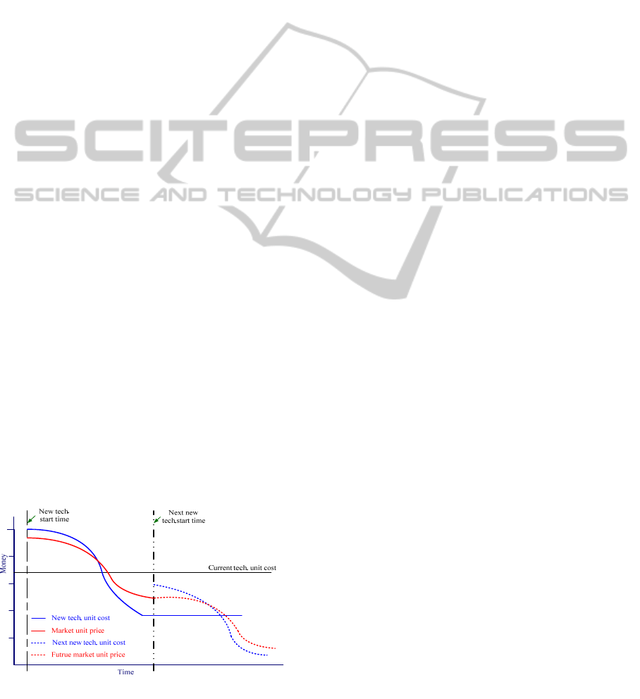
literature review and market survey, the trend of
DRAM unit cost and market price is as Fig. 1.
Because the equipment depreciation and product
yield is stable under the current production status,
the production cost of per giga bit DRAM is almost
the same. However, the market price will be dropped
off due to the business strategy, new product or
technology emerged. The trend of market price can
be gotten from history data. Regarding to the unit
cost produced by new technology, it will be higher
Figure 1: The relationship between unit cost and unit price
of per giga bit DRAM.
than current mature technology due to the higher
price of new equipment and lower yield of
production in the beginning. However, the yield will
be improved after a period of time and the unit cost
also can be dropped off and even lower than the
product from current technology. Based on the
abovephenomena, it shows that the best timing of
technology migration will be occurred between the
emerged time of new technology and the next
generation technology.
In order to analyse and establish the model easily,
we called the horizon between the emerged time of
new technology and the next generation technology
as the life cycle of new technology and divided it
into n periods. The profit function is established as
Eq. 1 and there are three parts, total revenue, total
manufacturing cost and the income of equipment
disposal, included. The details are described in the
follows.
∑
,
,
,
(1)
Where
:
Total profit which the technology
migrated from t period
:
The time of technology migration
:
Revenue of j generation technology
,
:
Fixed cost of g generation
technology per period which is
migrated at i period
:
Fixed cost of g-1 generation
technology per period
,
:
Variable cost of g generation
technology per period which is
migrated at i period
:
Variable cost of g-1 generation
technology per period
,
:
The income from the deposal of g-
1 generation equipment at t period
2.1 The Function of Total Revenue
The environment of supply demand balance is an
assumption of this work. Therefore, all products can
be sold by market price. The total revenue means the
revenue of n periods. If the new technology is
migrated at t period, the revenue from current
technology will be the revenue from period 1 to
period t-1 and the revenue from new technology will
be from period t to period n. Down below is the
ICEIS2013-15thInternationalConferenceonEnterpriseInformationSystems
390

equation of current technology revenue andnew
technology revenue.
2.1.1 The Revenue from Current Technology
If the current technology is not eliminated after new
technology emerged, the current technology is still
under production. Because the current technology is
under a stable stage, the market price and production
quantity of the company will keep almost the same.
Therefore, the revenue from current technology is
established as follows.
,
(2)
Where
:
The average market price of g-1
generation technology
,
:
The total quantity of g-1 generation
technology at period i
2.1.2 The Revenue from New Technology
The calculation of the revenue from new technology
is still formula by the price multiplying the quantity.
Due to the new technology belonging to the growing
stage, the market price and production quantity of
the company will be changed by time. Based on the
historical data analysis, the market price can be
modelled as a Sigmoid function. The output of
Sigmoid function is between 0 and 1. Therefore, the
managers should forecast the rate of price change
and the saddle point of price curve. Besides, the
normalization is used to fit the actual DRAM price.
Regarding to the production quantity, due to the
unfamiliarity of new technology process, the yield of
products will be lower in the beginning. After a
period of time, the yield can be improved and
products quantity will be increased as well. This
concept is similar to the learning curve. Therefore,
the concept of learning curve is applied to model the
production quantity of new technology. The
equation of the revenue from new technology is as
follows.
,
,
(3)
,
,
,
,
(4)
1
1
(5)
1
1
(6)
Where
,
:
The average price of g generation
technology at i period
,
:
The maximum price of g generation
technology
,
:
The minimum price of g generation
technology
:
The normalization value of Sigmoid
function
:
The rate of price change
:
The saddle point of Sigmoid function
:
Production quantity at i period
:
Release quantity per period
:
The initial failure rate of new
technology
:
The learning rate of production
failure rate, set by the managers
2.2 The Function of Total Cost
As the characteristics of DRAM industry, the
company can get more profit from new generation
technology. However, a huge of cost should be paid
for new generational equipment behind profit. This
cost is called as capacity acquired cost. Therefore,
the calculation of production cost can be divided
into two part, fixed cost and variable cost. The fixed
cost is the cost of equipment for new technology and
the depreciation of current equipment. There is no
depreciation for the deposal equipment. The variable
cost is the expense for the production. The details
are as follows.
2.2.1 Fixed Cost of New Technology
Due to the migration to new generational
technology, the new generational equipment is
required. Generally, the price of new generational
equipment will be reduced by time. In this work we
assume the price will be linear decreasing. Besides,
the required equipment quantity depends on its
throughput. Based on these concepts, the fixed cost
is formulized as follows.
,
,
(7)
,
,
1
(8)
,
(9)
TechnologyMigrationDeterminationModelforDRAMIndustry
391

,
1
(10)
(11)
Where
,
:
The quantity of generation g
equipment which purchased ati period
:
The reducing value of equipment per
period
,
The price of generation g equipment
which purchased at i period
The fixed cost of generation g-1
equipment which is disposed at period
t
:
The residual value of generation g
equipment
:
N
umbers of depreciation period
:
The capacity of generation g
equipment
:
The wafer numbers which producing
by the generation g equipment
:
The numbers of IC which producing
by the generation g equipment
:
The memory size per die which
producing by the generation g
equipment
2.2.2 Variable Cost of New Technology
Generally, the variable cost of production will
decrease as the yield increase. The yield increasing
is the result of the mature of co-operating in man-
machine and the accumulation of engineer’s
experiences. Therefore, the variable cost will present
same as the concept of manufacturing progress
function and it is applied in the formulation of
variable cost.
VC
,
C
it1
(12)
Where
:
The variable cost which the migration
occurred at
t
p
erio
d
:
The learning rate of variable cost, set
by
the mana
g
ers
2.3 The Income from the Disposal of
Equipment
The equipment which cannot process the new
generation technology will be disposed. The income
from the disposal of equipment is as the following
equation.
,
,
,
(13)
Where
,
:
The price of g-1 generationa
l
equipment at t period
,
:
The equipment quantity of g-1
generational equipment
3 NUMERICAL EXAMPLE
Here, a numerical example is illustrated to
demonstrate the modelling and determination
process of the proposed model. The environment of
this example is a 300mm DRAM fab with 30K
wafers per month. The major product is DDRII and
1300 chips per wafer. New generation technology is
DDRIII and 1800 chips per wafer. The sales quantity
is equal to the production quantity under the
assumption of strong market demand condition.
Besides, the duration of period is one month and all
cost, price and revenue are counted by US dollar.
The following is the detailed modelling and
determination process. Furthermore, t=8 is assumed
for all calculation.
3.1 Total Revenue
3.1.1 The Revenue from Current Technology
Assume the price of current technology is $0.8 per
giga bit and production yield is 0.98. Therefore, the
revenue from current technology is as follows.
R
1.2130030K0.98
45,864,0007
321,048,000
3.1.2 The Revenue from New Technology
Regarding to the price of DDRIII, the data from Aug.
2009 to July 2012 is collected to formula the
Sigmoid function. Assume the parameters of
Sigmoid function T is 16 and a is 0.3. The maximum
and minimum price of DDRIII is 2.5 and 1.2. The
price of new technology is as follows.
X
1
1e
.
0.9168
P
,
0.9168
2.51.2
1.22.3918
ICEIS2013-15thInternationalConferenceonEnterpriseInformationSystems
392

Due to the improvement of product yield, the
production quantity will increase. Assume the
product yield is 0.45 in the beginning of migration
and c
1
equals to 0.85. The production quantity of
period 8 is calculated as follows.
Q
,
54,000K
1
0.55
881
.
23,220,000
a
log0.9
log2
0.152
The revenue from new technology is as follows.
R
P
,
Q
,
1,504,087,017
3.2 Total Cost
3.2.1 Fixed Cost
Assume the depreciation for equipment is six years.
Three sets of g-1 generation should be replaced and
their original cost is 0.1 billion. Total equipment
cost of old technology excluding the disposals is 2
billion. The parameters of product by new and old
technology are as follows.
ICC
g
=1GB, CP
g
=1800, MP
g
=10000
ICC
g-1
=1GB, CP
g-1
=1300, MP
g-1
=10000
Therefore, C
g
and C
g-1
equals to 18,000,000 and
13,000,000. The new generational equipment
quantity can be determined by Eq. 10.
x
130000000.983
180000000.61
13
Assume the price of new generational equipment
is 1 billion per set in the beginning and its
residual
value is 0.2 billion. Therefore, if the new
generational equipment is purchased at period 8,
its price is calculated as follows.
100,000,00020,000,000
72
1,111,111
MP
,
100,000,0001,111,1117
$92,222,222
Based on the assumptions above, the total fixed
cost is calculated as follows.
FC
,
92,222,2223
72
2,000,000,000
72
31,620,370
,
,
1,121,157,407
3.2.2 Variable Cost
Assume c
2
= 0.82, C
t
=10,600,000 and VC
g-
1,i
=7,141,000
Then a
log0.82/log20.377069649
VC
10,600,000881
.
10,600,000
VC
,
156,956,539
The following is the calculation of total variable
cost.
VC
,
,
7,141,0007156,956,539
206,943,539
The total cost is fixed cost plus variable cost.
TotalCost1,121,157,407
206,943,5391,328,100,946
3.3 The Income from the Disposal of
Equipment
Assume the disposal equipment has been purchased
for 47 months at the time of new technology
emerged. Therefore, the total value at the period 8 is
as follows.
I
,
,,.
17100,000,0000.2
3
3
38,888,888
3.4 Total Profit
Finally the total profit is as follows if the technology
migration occurred at period 8.
TP
8
321,048,0001,504,087,017
1,328,100,94638,888,888
535,922,959
TechnologyMigrationDeterminationModelforDRAMIndustry
393
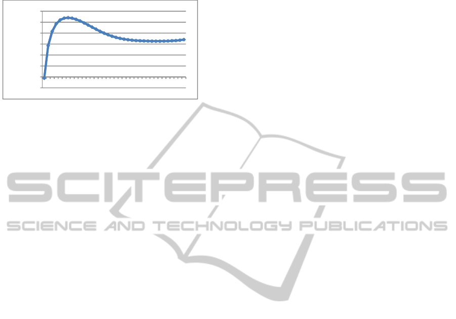
Based on the above calculation, the relationship of
total profit vs. the migration time t is shown as Fig. 2.
Figure 2: The relationship between total profit and
migration time t.
The best time for generational transition can be
determined as period 7 from Fig. 2.
4 CONCLUSIONS
DRAM industry is a capital intensive, high-tech
industry and the product generation has been quickly
enhanced. Due to the huge investment for the
technology migration, the migration timing is very
important for the company. In this work, a model to
determine the best timing for the technology
migration is established. The maximum profit is the
objective to determine the migration time in the
model. All revenue and cost of technology migration
are considered. We expect this model can be applied
in other industries with same situation.
ACKNOWLEDGEMENTS
The authors would like to thank the National Science
Council of the Republic of China for financially
supporting this research under Contract No. NSC 100-
2628-E-216-002-MY2.
REFERENCES
Cainarca, C. (1989). Dynamic Game Results of the
Acquisition of New Technology. Operations Research,
37(3), 410-425.
Chand, S. and Sethi, S. (1982). Planning Horizon
Procedures for Machine Replacement Models with
Several Possible Replacement Alternatives. Naval
Research Logistics Quarterly, 29(3), 483-493.
Chien, C. F. and Zheng J. N. (2011), Mini-max regret
strategy for robust capacity expansion decisions in
semiconductor manufacturing, Journal of Intelligent
Manufacturing DOI: 10.1007/s10845-011-0561-1, 1-9.
Chou, Y. C., Cheng, C. T., Yang F. C. and Liang, Y. Y.
(2007).Evaluating alternative capacity strategies in
semiconductor manufacturing under uncertain demand
and price scenarios, International Journal of
Production Economics, 105(2), 591-606
Cohen, M. A. and Halperin, R. M. (1986). Optimal
Technology Choice in a Dynamic Stochastic
environment. Journal of Operations Management,
6(3), 317-331.
Hastings, J. (1994). AmCoEx Five Year Comparison of
Used Computer Prices, Computer Currents, 9, 20-24.
Pak, D., Pornsalnuwat, N. and Ryan, S. M. (2004),The
effect of technological improvement on capacity
expansion for uncertain exponential demand with lead
times, The Engineering Economist: A Journal Devoted
to the Problems of Capital Investment, 49(2), 95-188.
Rajagopalan, S., Singh, M.R., and Morton, T.E.
(1998).Capacity expansion and replacement in
growing markets with uncertain technological
breakthroughs. Management Science, 44(1), 12-30.
Seta, M. D., Gryglewicz, S. and Kort, P. M. (2012),
Optimal investment in learning-curve technologies,
Journal of Economic Dynamics and Control, 36(10),
1462-1476.
‐100
0
100
200
300
400
500
600
1 3 5 7 9 11131517192123252729313335
Million
ICEIS2013-15thInternationalConferenceonEnterpriseInformationSystems
394
