A Rule Induction with Hierarchical Decision Attributes

Chun-Che Huang

, Shian-Hua Lin

, Zhi-Xing Chen

and You-Ping Wang

Department of Information Management, National Chi Nan University, #1, University Road, Pu-Li, Taiwan 545, Taiwan

Department of Computer Science and Information Engineering, National Chi Nan University,

#1, University Road, Pu-Li, Taiwan 545, Taiwan

Keywords: Concept Hierarchy, Rough Set Theory, Rule Induction, Decision Making.

Abstract: Hierarchical attributes are usually predefined in real-world applications and can be represented by a concept

hierarchy, which is a kind of concise and general form of concept description that organizes relationships of

data. To induct rules from the qualitative and hierarchical nature in data, the rough set approach is one of the

promised solutions in data mining. However, previous rough set approaches induct decision rules that

contain the decision attribute in the same hierarchical level. In addition, comparison of the reducts using the

Strength Index (SI), which is introduced to identify meaningful reducts, is limited to same number of

attributes. In this paper, a hierarchical rough set (HRS) problem is defined and the solution approach is

proposed. The proposed solution approach is expected to increase potential benefits in decision making.

1 INTRODUCTION

Rough Set (RS) theory was developed by Pawlak

(1982) to classify imprecise, uncertain, or

incomplete information, or knowledge expressed by

data acquired from experience (Pawlak, 1982). The

main advantage of rough set theory is that it does not

require any preliminary or additional information

about data: like probability in statistics or basic

probability assignment in Dempster–Shafer theory

and grade of membership or the value of possibility

in fuzzy set theory (Thangavel and Pethalakshmi,

2009). Over the past years, RST has indeed become

a topic of great interest to researchers and has been

applied in many areas.

Previous Rough Set (RS) Theory approaches

cannot produce rules containing preference order,

namely, cannot achieve more meaningful and

general rules (Sun et al., 2005). RS based induction

often generates too many rules without focus and

cannot guarantee that the classification of a decision

table is credible, for example, generation of

classification rules in Hassanien (2004),

information-rich data to reduce the data redundancy

in Jensen and Shen (2004), the analysis of diabetic

databases in Breault (2001), an unsupervised

clustering in Questier et al., (2002), discovery of

statistical significance rules in Yin et al., (2001), and

an algorithm to infer rules in Phuong et

al., (2001).

Tseng (2008) proposed a new RS method, called

alternative rule extraction algorithm (AREA) to

discover preference-based rules according to the

reducts with the maximum of strength index (SI),

which is introduced in order to identify meaningful

reducts. However, comparison of the reducts using

the Strength Index (SI) is limited to the same

number of attributes. SI should be counted in a

reasonable way of average the weights of selected

attributes.

Moreover, Tseng (2008) and most of the

previous studies on rough sets focused on finding

rules that a decision attribute does not have

hierachical concept. However, hierarchical attributes

are usually predefined in real-world applications and

could be represented though a hierarchy tree (Hong

et al., 2009). A concept hierarchy is a kind of

concise and general form of concept description that

organizes relationships of data.

In this study, a hierarchical rough set (HRS)

problem is defined as follows: Given a decision

table data with hierarchical decision attributes, one

could induct decision rules from the reducts, the

minimal subset of attributes that enables the same

classification of elements of the universe as the

whole set of attributes in each corresponding object.

The reduct has the highest strong index (SI).

The objective of this study is to develop a

Huang C., Lin S., Chen Z. and Wang Y..

A Rule Induction with Hierarchical Decision Attributes.

DOI: 10.5220/0004410900950102

In Proceedings of the 15th International Conference on Enterprise Information Systems (ICEIS-2013), pages 95-102

ISBN: 978-989-8565-59-4

 2013 SCITEPRESS (Science and Technology Publications, Lda.)

solution approach to resolve the HRS problem based

on AREA and characterized:

1) Induct a reduct that is the minimal subset of

attributes that enables the same classification of

elements of the universe as the whole set of

attributes.

2) Present a revised strength index to identify

meaningful reducts from all reducts, rather than

from the same number of attributes selected in the

reducts.

3) Explore the most specific decision attribute level

by level in the level-search procedure.

The paper is outlined as follows: Section 2 surveys

the literature related to rough set theory. Section 3

proposes the solution approach and section 4

concludes this study.

2 LITERATURE REVIEW

Rough sets theory has often proved to be an

excellent mathematical tool for analyzing a vague

description of objects (called actions in decision

problems). The adjective “vague”, refers to the

quality of information and means inconsistency or

ambiguity which follows from information

granulation (Pawlak, 1982). In the Rough Set (RS)

Theory, a reduct is the minimal subset of attributes

enabling the same classification of elements of the

universe as the whole set of attributes. In the RS

theory, attributes are classified into two sets:

condition and decision attributes. The second one

refers to the outcomes of the data set. Rough sets

theory has often proved to be an excellent

mathematical tool for analyzing a vague description

of objects (called actions in decision problems). The

adjective “vague”, refers to the quality of

information and means inconsistency or ambiguity

which follows from information granulation

(Pawlak, 1982; 1991).

Over the past years, the RS theory has indeed

become a topic of great interest to researchers and

has been applied to many areas, for example,

environmental performance evaluation (Chèvre et

al., 2003); (Yang et al., 2011), machine tools and

manufacture (Jiang et al., 2006), industrial

engineering (Liu et al., 2007), integrated circuits

(Yang et al., 2007), medical science (Pattaraintakorn

and Cercone, 2008); (Salama, 2010), economic and

financial prediction (Chen and Cheng, 2012);

(Cheng et al., 2010); (Tay and Shen, 2002),

electricity loads (Pai and Chen, 2009),

meteorological (Peters et al., 2003), airline market

(Liou and Tzeng, 2010) customer relationship

management (Tseng and Huang, 2007),

transportation (Kandakoglu et al., 2009); (Léonardi

and Baumgartner, 2004); (Utne, 2009) and other

real-life applications (Lewis and Newnam, 2011);

(Sikder and Munakata, 2009); (Yeh et al., 2010).

This success is due in part to the following aspects

of RS theory: (i) Only the facts hidden in data are

analyzed, (ii) No additional information about the

data is required such as thresholds or expert

knowledge, and (iii) A minimal knowledge

representation can be attained (Jensen and Shen,

2004).

However, previous studies on rough sets focused

on finding certain rules and possible rules that a

decision attribute is in one level only and not

hierarchical. However, hierarchical attributes are

usually predefined in real-world applications and

could be represented by a hierarchy tree (Hong et al.,

2009). A concept hierarchy is a kind of concise and

general form of concept description that organizes

relationships of data. Tseng (2006) proposed an

approach to generate concept hierarchies for a given

data set with nominal attributes based on rough set.

Dong et al., (2002) presented the model and

approach for hierarchical fault diagnosis for

substation based on rough set theory. These

approaches not only improve the efficiency of the

discovery process, but also express the user's

preference for guided generalization. However, they

did not consider the decision attribute with different

values in a different level combination, for example,

outcome O1 at level 1, outcome O2 at level 2, and

O3 at level 2.

Moreover, traditional RS approaches cannot

produce rules containing preference order, namely,

cannot achieve more meaningful and general rules

(Sun et al., 2005). RS based induction often

generates too many rules without focus and cannot

guarantee the classification of a decision table is

credible. For example, generation of classification

rules in Hassanien (2004), information-rich data to

reduce the data redundancy in Jensen and Shen

(2004), the analysis of diabetic databases in Breault

(2001), an unsupervised clustering in Questier et al.,

(2002), discovery of statistical significance rules in

Yin et al., (2001), an algorithm to infer rules in

Phuong et al. (2001).

New approaches, e.g., Tseng (2008) proposed a

new RS method, called alternative rule extraction

algorithm (AREA) to discover preference-based

rules according to the reducts with the maximum

strength index (SI), which is introduced to identify

meaningful reducts. However, these approaches used

ICEIS2013-15thInternationalConferenceonEnterpriseInformationSystems

two stages to generate reducts and induct decision

rules, respectively. Large computing space is

required to store the reducts from the first stage, and

solution searching is complex. Moreover,

comparison of the reducts using SI is limited to the

same number of condition attributes which are

selected in the reducts.

Next, a hierarchical decision rule induction

algorithm was proposed to solve the hierarchical

rough set (HRS) problem defined in section 3.

3 SOLUTION APPROACH

The hierarchical rough set problem is defined in this

section first. The concept of the hierarchy

framework is introduced and three axioms are

presented to show how the optimal level decision

rules are reached. The hierarchical decision rule

induction algorithm (HDRIA) is proposed to find the

decision rules finally. The accuracy and the

coverage are presented for each decision rule by

HDRIA.

3.1 Hierarchical Rough Set (HRS)

Problem

In this study, the hierarchical rough set problem is

defined as:

Given:

1) A hierarchical transportation decision table I =

(U, A∪{d}), where U is a finite set of objects and A

is a finite set of attributes. The elements of A are

called condition attributes. d ∉ A is a distinguished

hierarchical decision attribute at different level.

2) A concept hierarchy (a tree or a lattice) Hk refers

to on a set of domains Ox,…,Oz:

Hksk:{Ox …Oz} → Hksk-1 → Hk1, where

Hksk denotes the set of concepts at the the skth

level, Hksk-1 denotes the concepts at one level

higher than those at Hksk , and Hk1

represents the top level denoted as “ANY”.

Objective:

Minimize the subset of U, in which the specific

decision attribute of decision rules (ri) is with the

highest Strong Index (SI) and maximal level

number.

Subject to the following four constraints:

1) A = C



2) B



3) POSB(D) = {x



U: [x]B



4) For any a



B of C, K (B, D) = K (C, D), and

K (B, D)



K(B-{a}, D), where, C is condition

domain and D is decision domain. Attribute a ∈ A,

set of its values. K(B, D) is the degree of

dependency between B and D.

))D(POS(card

)D,B(K



POSB(D) is the positive region and includes all

objects in U which can be with classified into classes

of D, in the knowledge B.

3.2 The Structure of the Concept

Hierarchies

Notation:

O: a decision attribute set;

k: decision attribute hierarchical index;

l: level index;

e: entry point;

Hk: the concept hierarchy corresponding to O;

Hkl: the concept hierarchy corresponding to O at

level l;

sk: number of levels in the Hk;

Suppose that a concept hierarchy Hk refers to on a

set of domains Ox,…,Oz. Hksk:{Ox ×…×Oz} →

Hksk-1 → Hk1, where Hksk denotes the set of

concepts at the skth level, Hksk-1 denotes the

concepts at one level higher than those at

Hksk , Hk1 represents the top level denoted as

“ANY”, Ox refers to the value of attribute = x at

level 1, Ox.y refers to the value of attribute = x at

level 1 and y at level 2, and Ox.y.z refers to

the value of attribute = x at level 1, y at level 2, and

z at level 3, …, etc.

Ox.y.z ∈ Ox.y ∈ Ox implies that more level, more

specific information. And, in the concept tree, Ox is

father node of Ox.y. Ox.y is a son node of Ox. Ox.y

and Ox.n are brother node for each other.

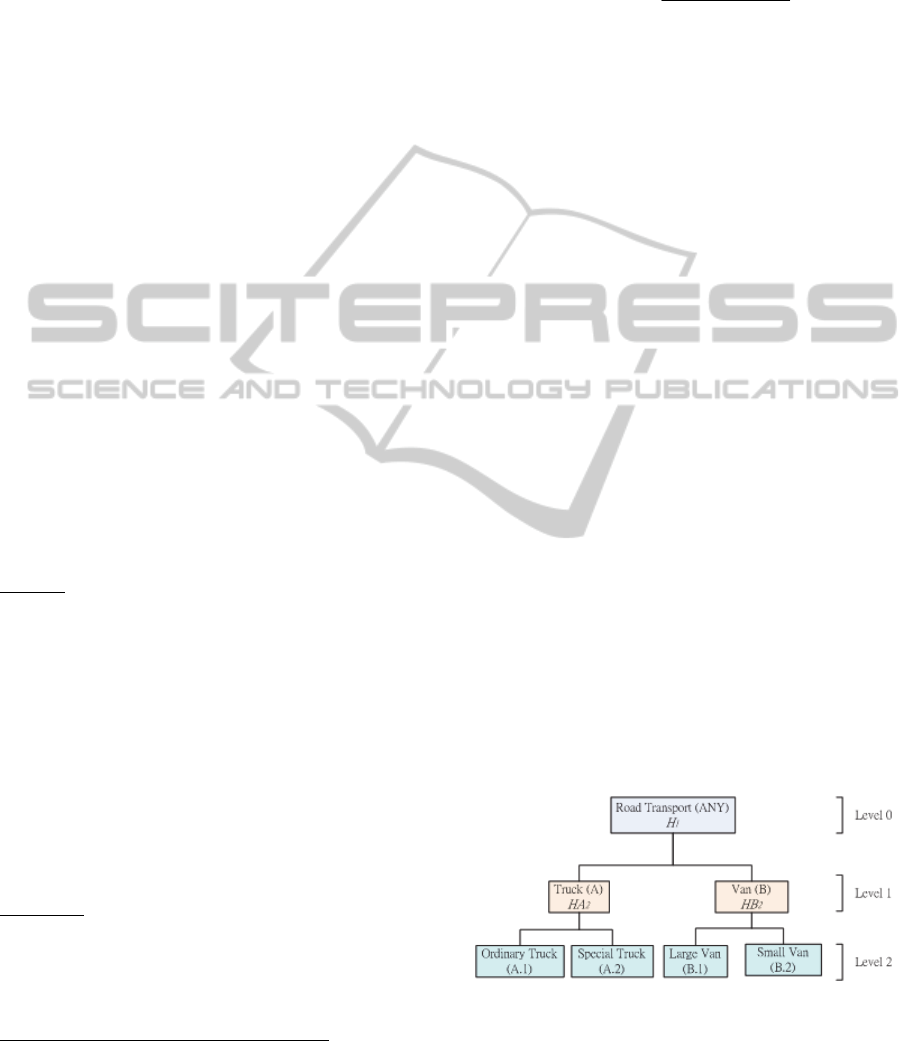
Figure 1: An example of Concept Tree.

In the concept tree, the most general concept can

be a universal concept, whereas the most specific

concepts correspond to the specific values of

attributes in the data set. Each node in the tree of

ARuleInductionwithHierarchicalDecisionAttributes

concept hierarchy represents a concept

transportation hierarchy. In Fig. 1, for example,

OA.1 ∪ OA.2 = HA2 ∈ OA, OB.1 ∪ OB.2 =

HB2 ∈ OB, OA ∪ OB = H1 ∈ O0.

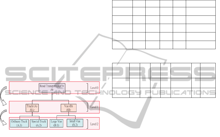
3.3 The Level-search Procedure

Three axioms are supported to show how the final

decision rules are reached. Initially, the default entry

point for hierarchical decision attribute (outcome) is

at the top level (e =1). Then the level-search

procedure explores down level until violation from

the axioms to stop further exploration. The final

decision rules are induct.

For example, in Fig. 2, the decision rule’s

outcome at Level 2 (OA.2 = the special truck) is

more informative than Level 1 (OA = truck). The

procedure will explore level 2 if no any violation in

three axioms.

Figure 2: Concept hierarchies search process.

The three axioms are proposed as follows:

Notations:

O: a decision attribute (outcome) set;

k: the decision attribute hierarchical index;

L: level of concept hierarchy;

l: level index;

Ck: the node of outcome Ok in the concept

hierarchy

Hkl.

Axiom 1: Ll is more informative than Ll-1

Axiom 2: For the node Ck in the hierarchy tree,

outcome of each Ck’s children nodes ∉ outcomes

of all current decision rule set, stop explore.

Axiom 3: Stop exploring node Ck if two conditions

are met: (1) its outcome Ok ∈ outcomes in current

decision table, but ∉outcome of the current

decision rule set. (2) Outcomes in its brother node ∈

outcomes in current decision table, and ∈outcomes

of the current decision rule set.

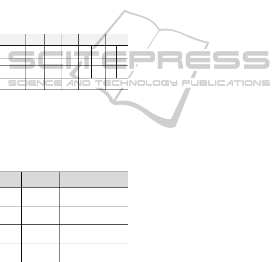
For example, given a decision table in Table I, The

outcomes are explored at level 2. There are three

outcomes (1.1, 1.2, and 2.1). The data of the level 2

decision table are exemplified in Table I. Apply the

RS approach and explore at a node C1, the current

decision rule set is obtained in Table II.

Table 1: The level 2 decision table.

Object A1 A2 A3 O Cardinal number

1 1 2 2 1.1 10

2 2 2 1 1.1 10

3 2 2 1 1.2 10

4 1 1 1 2.1 10

Wj 0.1 0.4 0.2

Table 2: The level 2 decision rule set.

Rule NO A1 A2 A3 O

Object

Cardinality

Support

Object

2 1.1 10 2 1

2.1 10 4 4

Object 3 has the outcome O

1.2

in the decision

table but not in the current decision rule set.

Moreover, the outcome O

1.2

who has brother

outcome O

1.1

is in the decision table and also in the

decision rule. Then, stop exploring node C

. In this

case, since two outcomes of brother nodes conflict to

each other (i.e. one of them is not in the decision set),

the procedure will stop at their father node.

3.4 The Hierarchical Decision Rule

Induction Algorithm (HDRIA)

The main idea of the HDRIA is to select an object to

entry. Then set the default entry point e = L1 and

CANCk = GO. Based on DREA in Section II-A,

find the set of decision rules for each object. For

each note Ck, if CANCk = GO then check:

According to Hkl, if all outcomes of decision table ∈

outcomes of the current decision rule set, based on

Axiom 1, then explore next level.

According to Hkl, if all outcomes of decision table

∉ in outcome of decision rule, based on Axiom 2,

then stop exploring this node.

According to Hkl, if the node Ckl whiose outcomes

(Ok) in the Hkl corresponding decision table ∉

outcomes of the current decision rule set, but there

is another brother note Ck’l whose outcome (Ok’) of

the corresponding decision table ∈ the current

decision rule set, then based on Axiom 3, stop

exploring Ckl. And go exploring its brother node,

ICEIS2013-15thInternationalConferenceonEnterpriseInformationSystems

Ck’l.

If Ckl has no more low level, then stop explore,

otherwise repeat these steps until no more node to

explore.

In the AREA proposed by Tseng (2008), the strength

index of reduct f is computed as SI(f) =





j 1

* n

The weakness of the that SI(f) is the comparison of

the reducts is limited to the same decision attribute

and to same number of attributes selected in the

reducts. While number of attributed involved is

more, the SI(f) is larger, which conflicts with the

objective of an attribute reduct which is a minimal

subset of attributes that provides the same

descriptive ability as the entire set of attributes. In

the other words, attributes in a reduct is jointly

sufficient and individually necessary (Yao and Zhao,

2009). Therefore, the SI(f) is revised and refers to as

follows:

SI(f) =





j 1







j 1



(1)

where: f is the reduct index, f = 1, ..., n;

= 1 if condition attribute j is selected,

0 otherwise (A

= “x”);

is the weight of condition attribute j;

is the number of identical reducts f;

The hierarchical decision rule induction algorithm

(HDRIA) is presented as follow:

Notation:

e: entry point;

L: level of concept hierarchy;

l:l evel index;

O: a decision attribute set;

k: decision attribute hierarchical index;

Hk: the concept hierarchy corresponding to Ok;

Hkl: the concept hierarchy corresponding to Ok

at level

Ckl: the node of outcome Ok in the concept

hierarchy

Hkl;

CAN





: an option GO or NG for Ckl. GO means

can go

to next level. NG means stop;

r: node index;

sk: number of levels in the Hk;

sr: number of Ckl;

Input: the decision table

Output: the decision rule set

Step 0 Initialization

Select the block of the data need to

analysis.

Set the default entry point e = L1.

Set 





= GO

Step 1 Based on Axiom 1

For l = 1 to sk+1

Apply DRIA to find the decision rule

set

For r = 1 to sr

If CAN





= GO

If all Hk

outcomes of decision table ∈

outcomes of all decision rules then set 





← GO

End if

If all Hk

outcomes of decision table ∉ outcome

of decision rule

Based on Axiom 2, then set 





← NG

End if

If node Ck

in Hk

outcome (O

) of decision table

∉ outcome of decision rule, but other node Ck

outcome (O

k’

) of decision table ∈ the

decision rule set, then based on Axiom 3, set







← NG, 







← GO

Endif

Else If node Ck

no more relatively low level,

then Ck

= Ck

l-1

and 





← NG

End if

Else if 





= NG, then Stop;

End for

Step 2 Termination: Stop and output the results.

3.5 Validation of HDRIA

In order to validate the accuracy and coverage of

HDRIA, two performance measures are introduced:

accuracy index, coverage index. Accuracy index







and coverage index ψ







are defined as

following (Tsumoto, 1998):













|







∩

|







, and 0









1













|







∩



, and 0









1

where: |A| denotes the cardinality of set A, α







denotes the accuracy of R (e.g., eij = vij, in a

decision table) as to categorization of D, and ψ







denotes a coverage, respectively.

The accuracy (ac) and the coverage (co) of the

ARuleInductionwithHierarchicalDecisionAttributes

example (data in Table I and concept tree in Fig. 1)

are computed. The comparison between the optimal

level and all in top, 2

, 3

, and all in lowest levels

by HDRIA is presented in Table III. In Table III, the

coverage is the worst at the top level (the traditional

RS approaches). And the result of the coverage is

the best at the optimal level (the proposed approach).

The proposed algorithm can reach a final rule set,

which shows:

All qualified decision rules can be found.

The optimal level outcome is specific.

The best accuracy and coverage for each rule.

Table 3: The accuracy and coverage.

Top

level

The lowest

level

Optimal

level

Rule No. ac co ac co ac ac ac co ac co

1 0.5 0.33 1 1 1 1 1 1 1 1

2 1 0.67 1 1 1 1 1 1 1 1

3 1 0.5 1 0.5 1 1 - - 1 1

4 1 0.5 - - - - - - 1 1

Number of

rules

4 3 3 2 4

*Note: the lowest level refers that all outcomes are the specific in

the decision table.

The complexity of AREA and REA are

compared in Table IV. The results shows that REA

is more efficient since complexity of traditional RS

approach is O(n

) (Reduct Generation) + 3





 (REA). Complexity of REA algorithm is O(n

)

and HDRIA is   1



2





Table 4: The complexity of the proposed algorithms and

the original algorithms.

Algorithm Description Time complexity in the worst case

Reduct

Generation

Generate the reduct

from the decision

table.







AREA

Extract the decision

rule from the

reduct.

3





DRIA

Induct the decision

rule from the

decision table.





2





HDRIA

Find the final level

by DRIA

  1



2





where

n: total number of objects;

m: total number of attributes;

r: total number of reducts;

R: total number of decision rules;

sk: total number of levels;

4 CONCLUSIONS AND FUTURE

WORK

This study considered the hierarchical attributes that

are usually predefined in real-world applications by

a concept hierarchy concept tree. This study aimed

the decision maker to solve the hierarchical rough

set (HRS) problem and with the following

contribution:

1) Presented a revised strength index to identify

meaningful reducts from all reducts, rather than

from same number of attributes selected in the

reducts.

2) The (HDRIA) algorithm was proposed to

explore the decision rules of the hierarchical

decision attributes in different levels combination.

In the future, the condition attributes may consider

hierarchy concept, too. The extension to other

industry involving in the hierarchical and qualitative

data analysis is required. Also, a practical case will

be studied: The ABC company established in 1954

owns a fleet over 3000 vehicles, including trucks

and vans in different sizes. The fleet can be

developed in a hierarchy concept. The company

plans the daily scheduling that requires allocating

different types of vehicles according to different

routes. The solution is influenced by several factors,

including environmental regulations, which affect

the determination of the ratio of green vehicles in the

fleet. The ratio is a crucial reference in purchasing

new fleets. In this case study, selection of the

transportation fleet and determine the ratio is

undoubtedly the urgent problem that the ABC

company faces. Applying the proposed solution

approach to induct decision rules will aim resolving

the problem and enhancing the agility of decision

making.

REFERENCES

Breault, J. L., 2001. Data mining diabetic databases: are

rough sets a useful addition? Proceedings of the

Computing Science and Statistics, 33.

Chèvre, N., Gagné, F., Gagnon, P., and Blaise, C., 2003.

Application of rough sets analysis to identify polluted

aquatic sites based on a battery of biomarkers: a

comparison with classical methods. Chemosphere,

51(1), p.13-23.

Chen, Y. S., and Cheng, C. H., 2012. A soft-computing

ICEIS2013-15thInternationalConferenceonEnterpriseInformationSystems

100

based rough sets classifier for classifying IPO returns

in the financial markets. Applied Soft Computing,

12(1), p.462-475.

Cheng, C. H., Chen, T. L., and Wei, L. Y., 2010. A hybrid

model based on rough sets theory and genetic

algorithms for stock price forecasting. Information

Sciences, 180(9), p.1610-1629.

Dong, H., Zhang, Y., and Xue, J., 2002. Hiearchical fault

diagnosis for substation based on rough set.

Proceedings of the Power System Technology, 4,

p.2318–2321.

Hong, T. P., Liou, Y. L., and Wang, S. L., 2009. Fuzzy

rough sets with hierarchical quantitative attributes.

Expert Systems with Applications, 36(3, Part 2),

p.6790-6799.

Hassanien, E., 2004. Rough set approach for attribute

reduction and rule generation: a case of patients with

suspected breast cancer. Journal of the American

Society for Information Science and Technology,

55(11), p. 954–962.

Jiang, Y. J. Chen, J. and Ruan, X. Y., 2006. Fuzzy

similarity-based rough set method for case-based

reasoning and its application in tool selection.

International Journal of Machine Tools and

Manufacture, 46(2), p.107-113.

Jensen R. and Shen, Q., 2004. Fuzzy–rough attribute

reduction with application to web categorization,

Fuzzy Sets and Systems, 141(3), p.469-485

Kandakoglu, A., Celik, M., and Akgun, I., 2009. A

multi-methodological approach for shipping registry

selection in maritime transportation industry.

Mathematical and Computer Modelling, 49(3–4),

p.586-597.

Liou, J. J. H., and Tzeng, G. H., 2010. A

Dominance-based Rough Set Approach to customer

behavior in the airline market. Information Sciences,

180(11), p.2230-2238.

Liu, M., Shao, M., Zhang, W., and Wu, C., 2007.

Reduction method for concept lattices based on rough

set theory and its application. Computers Mathematics

with Applications, 53(9), p.1390-1410.

Léonardi, J., and Baumgartner, M., 2004. CO2 efficiency

in road freight transportation: Status quo, measures

and potential. Transportation Research Part D:

Transport and Environment, 9(6), p.451-464.

Lewis, I., and Newnam, S., 2011. The development of an

intervention to improve the safety of community care

nurses while driving and a qualitative investigation of

its preliminary effects. Safety Science, 49(10),

p.1321-1330.

Pawlak, Z., 1982. Rough Sets. International Journal of

Computer and Information Sciences, 11(5), p. 341-356

Pawlak, Z., 1991. Rough Sets: Theoretical Aspects of

Reasoning about Data. Kluwer Academic Publishers,

Boston.

Pai, P. F., and Chen, T. C., 2009. Rough set theory with

discriminant analysis in analyzing electricity loads.

Expert Systems with Applications, 36(5), p.8799-8806.

Peters, J. F., Suraj, Z., Shan, S., Ramanna, S., Pedrycz, W.,

and Pizzi, N., 2003. Classification of meteorological

volumetric radar data using rough set methods.

Pattern Recognition Letters, 24(6), p.911-920.

Pattaraintakorn, P., and Cercone, N., 2008. Integrating

rough set theory and medical applications. Applied

Mathematics Letters, 21(4), p.400-403.

Phuong, N. H., Phong, L. L., Santiprabhob P. and Baets,

B. De., 2001. Approach to generating rules for expert

systems using rough set theory. Proceedings of IEEE

International Conference on IFSA World Congress

and 20th NAFIPS, Vancouver, BC, Canada, 2,

p.877–882.

Questiera, F., Arnaut-Rollier, I., Walczak B. and Massart,

D. L., 2002. Application of rough set theory to feature

selection for unsupervised clustering. Chemometrics

and Intelligent Laboratory Systems, 63(2), p.155–167.

Sun, C. M., Liu, D. Y., Sun, S. Y., Li, J. F. and Zhang, Z.

H., 2005. Containing order rough set methodology.

Proceedings of 2005 International Conference on

Machine Learning and Cybernetics, Guangzhou,

China, 3, p.1722–1727.

Sikder, I. U., and Munakata, T., 2009. Application of

rough set and decision tree for characterization of

premonitory factors of low seismic activity. Expert

Systems with Applications, 36(1), p.102-110.

Tsumoto, S., 1998. Automated extraction of medical

expert system rules from clinical databases based on

rough set theory. Information Sciences, 112(1–4),

p.67-84.

Tseng, T. L., Huang, C. C., Jiang, F., and Ho, J. C., 2006.

Applying a hybrid data mining approach to prediction

problems: A case of preferred suppliers prediction,

International Journal of Production Research, 44(14),

p.2935-2954.

Tseng, T. L., Huang, C. C., 2007. Rough set-based

approach to feature selection in customer relationship

management. Omega, 35(4), p.365-383.

Tseng, T. L. B., Huang C. C. and Ho, J. C., 2008.

Autonomous Decision Making in Customer

Relationship Management: A Data Mining Approach.

Proceeding of the Industrial Engineering Research

2008 Conference, Vancouver, British Columbia,

Canada.

Tay, F. E. H., and Shen, L., 2002. Economic and financial

prediction using rough sets model. European Journal

of Operational Research, 141(3), p. 641-659.

Thangavel, K. and Pethalakshmi, A., 2009.Dimensionality

reduction based on rough set theory: A review Article,

Applied Soft Computing, 9(1), p.1-12.

Utne, I. B., 2009. Life cycle cost (LCC) as a tool for

improving sustainability in the Norwegian fishing fleet.

Journal of Cleaner Production, 17(3), p.335-344.

Yin, X., Zhou, Z., Li, N. and Chen, S., 2001. An Approach

for Data Filtering Based on Rough Set Theory.

Lecture Notes in Computer Science, 2118, p. 367-374.

Yeh, C. C., Chi, D. J., and Hsu, M. F., 2010. A hybrid

approach of DEA, rough set and support vector

machines for business failure prediction. Expert

Systems with Applications, 37(2), p.1535-1541.

Yao, Y. and Zhao Y., 2009. Discernibility matrix

ARuleInductionwithHierarchicalDecisionAttributes

101

simplification for constructing attribute reducts.

Information Sciences, 179(7), p.867-882.

Yang, M., Khan, F. I., Sadiq, R., and Amyotte, P., 2011. A

rough set-based quality function deployment (QFD)

approach for environmental performance evaluation: a

case of offshore oil and gas operations. Journal of

Cleaner Production, 19(13), p.1513-1526.

Yang, H. H., Liu, T. C., and Lin, Y. T., 2007. Applying

rough sets to prevent customer complaints for IC

packaging foundry. Expert Systems with Applications,

32(1), p.151-156.

ICEIS2013-15thInternationalConferenceonEnterpriseInformationSystems

102