
Sliding Mode Slip Suppression Control of Electric Vehicles
Shaobo Li
1
and Tohru Kawabe
2
1
Department of Computer Science, Graduate School of Systems and Information Engineering,
University of Tsukuba, Tsukuba 305-8573, Japan
2
Faculty of Engineering, Information and Systems, University of Tsukuba, Tsukuba 305-8573, Japan
Keywords:
Electric Vehicle, Slip Ratio, Sliding Mode Control, Energy Saving.
Abstract:
In this paper, a new SMC (sliding mode control) method for the slip suppression control of EVs (electric
vehicles) is proposed. The proposed method aims to improve the maneuverability, the stability and the low
energy consumption of EVs by controlling the wheel slip ratio. The proposed method is the extended SMC
method adding the integral term to improve the control performance. There also include numerical simulation
results to demonstrate the effectiveness of the method.
1 INTRODUCTION
In recent years, Electric Vehicles (EVs) have attracted
great interests as a powerful solution against the en-
vironment and energy problems(Brown et al., 2010;
Mousazadeh et al., 2009; Hirota et al., 2011; Kondo,
2011).
EVs are automobiles which are propelled by elec-
tric motors, using electrical energy stored in batteries
or another energy storage devices. Electric motors
have several advantages over (internal-combustion
engines) ICEs:
• Energy efficient. Electric motors convert 75% of
the chemical energy from the batteries to power
the wheels - ICEs only convert 20% of the energy
stored in gasoline.
• Environmentally friendly. EVs emit no tailpipe
pollutants, although the power plant producing
the electricity may emit them. Electricity from
nuclear-, hydro-, solar-, or wind-powered plants
causes no air pollutants.
• Performance benefits. Electric motors provide
quiet, smooth operation and stronger acceleration
and require less maintenance than ICEs.
• Reduce energy dependence. Electricity is a do-
mestic energy source.
The travel distance per charge for EV has been in-
creased through battery improvements and using re-
generation brakes, and attention has been focused on
improving motor performance. The following facts
are viewed as relatively easy ways to improve maneu-
verability and stability of EVs.
1. The input/output response is faster than for gaso-
line/diesel engines.
2. The torque generated in the wheels can be de-
tected relatively accurately
3. Vehicles can be made smaller by using multiple
motors placed closer to the wheels.
Much research has been done on the stability of
general automobiles, for example, ABS (Anti-lock-
Braking Systems), TCS (Traction-Control-Systems),
and ESC (Electric-Stability-Control)(Zanten et al.,
1995) as well as VSA (Vehicle-Stability-Assist)(Kin
et al., 2001) and AWC (All-Wheel-Control) (Sawase
et al., 2006). What all of these have in common is
that they maintain a suitable tire grip margin and re-
duce drive force loss to stabilize the vehicle behavior
and improve drive performance.
When the vehicle is starting off or accelerating,
particularly on a slippery or wet road surface, the
wheel spins easily, which causes unstable driving sit-
uation and large waste of energy. Therefore, it’s im-
portant to keep the optimal driving force in all driving
situation for motion stability and saving energy. Dur-
ing acceleration, the driving force of wheel directly
depends on the friction coefficient between road and
tire, which is in accordance with the wheel slip and
road conditions. For this reason, it becomes possible
to give the adequate driving force by controlling the
wheel traction.
Several methods have been proposed for the trac-
11
Li S. and Kawabe T..
Sliding Mode Slip Suppression Control of Electric Vehicles.
DOI: 10.5220/0004411000110018
In Proceedings of the 10th International Conference on Informatics in Control, Automation and Robotics (ICINCO-2013), pages 11-18
ISBN: 978-989-8565-71-6
Copyright
c
2013 SCITEPRESS (Science and Technology Publications, Lda.)

tion control by using slip ratio of EVs (Kodama et
al., 2004), (Mubin et al., 2006), (Fujii and Fujimoto,
2007), such as the method based on Model Follow-
ing Control (MFC) in (Hori, 2000) and Model Predic-
tive PID method (MP-PID) in (Kawabe et al., 2011).
Both of these methods show good performances un-
der the nominal conditions where the situation, for
example, mass of vehicle, road condition, and so on,
is not changed. To meet the high performance even
variation happened in the conditions, it is significant
to construct the robust method against the situation
changing. About this point, Sliding Mode Control
(SMC) has been performed good robustness for the
systems with uncertainties or nonlinearities. How-
ever, for slip ratio control with the conventional SMC,
the control performance will get degradation due to
the chattering which always occurs because of switch-
ing the control inputs due to the structure of SMC. To
overcome such disadvantages of conventional SMC
method, new SMC method with introducing the inte-
gral term to the design of the sliding surface in order
to get better control performance and save more en-
ergy for slip suppression of EVs with changing the
mass of vehicle and road condition is proposed. The
numerical examples show the effectiveness of the pro-
posed method.
2 PRELIMINARIES OF SMC
Consider the single input nonlinear system (Slotine et
al., 1991)
x
(n)
= f (x) + b(x)u (1)
where x =
x ˙x ... x
(n−1)
T
is the state vector and u is
the control input. In general, the function f (x) and
the control gain b(x) are not exactly known but the
extents of the imprecision on f (x) and b(x) are upper
bounded by known. The control problem is to seek
a solution that is robust to uncertainties in f (x) and
b(x). Firstly, we defined a time-varying surface s(x;t)
in the state space R
(n)
by
s(x;t) =
d
dt
+ α
n−1
˜x = 0, α > 0 (2)
where ˜x = x − x
∗
=
˜x
˙
˜x ... ˜x
(n−1)
T
is the error be-
tween the output state x and the desired state x
∗
. The
problem of tracking x = x
∗
is equivalent to remain-
ing on the surface s for all t > 0. When s = 0, that
is to say, the output state reaches the surface which
represents the error is zero. Here, s = 0 is called slid-
ing surface. On this surface the error will converge to
zero exponentially. When ˙s = 0, the state is controlled
to slide on the sliding surface, which is described that
the system is in sliding mode.
The SMC law contains two parts, the equivalent
control u
eq
and the hitting control u
ht
, which is de-
fined as follows,
u = u
eq
+ u
ht
. (3)
u
eq
can be interpreted as the continuous control law
which would maintain ˙s = 0 when the dynamics are
exactly known. When the dynamics are not exactly
known, such as the uncertainties occur in the system
or the state of system is off the sliding surface, u
ht
acts to bring the state back to the sliding surface and
keeps it in sliding mode. Generally, u
ht
uses a dis-
continuous function to realize the switching action on
sliding surface.
For choosing the control input u, it is necessary
to consider the sliding condition (Eker and AKinal,
2008), which is defined as
1
2
d
dt
s
2
≤ −η|s| (4)
where η > 0. From eq. (4) , s
2
shows that the squared
“distance” to the sliding surface, which decreases
along all system trajectories. Particularly, once the
states reach the surface, the system trajectories remain
on the surface. In other words, satisfying the sliding
condition makes the trajectories reach the surface in
finite time, and once on the manifold, it cannot leave
it. Furthermore, eq. (4) also implies that some dy-
namic uncertainties can be tolerated while still keep-
ing the surface an invariant set.
To realize the concept of SMC, we always need to
follow two steps:
[Step 1 ] Design a sliding surface s which is invari-
ant of the controlled dynamics.
[Step 2 ] Choose the control input u which drives the
states to the sliding surface in sliding mode in fi-
nite time.
3 ELECTRIC VEHICLE
DYNAMICS
As a first step toward practical application, this paper
restricts the vehicle motion to the longitudinal direc-
tion and uses direct motors for each wheel to simplify
the one-wheel model to which the drive force is ap-
plied. In addition, braking was not considered this
time with the subject of the study being limited to
only when driving.
ICINCO2013-10thInternationalConferenceonInformaticsinControl,AutomationandRobotics
12
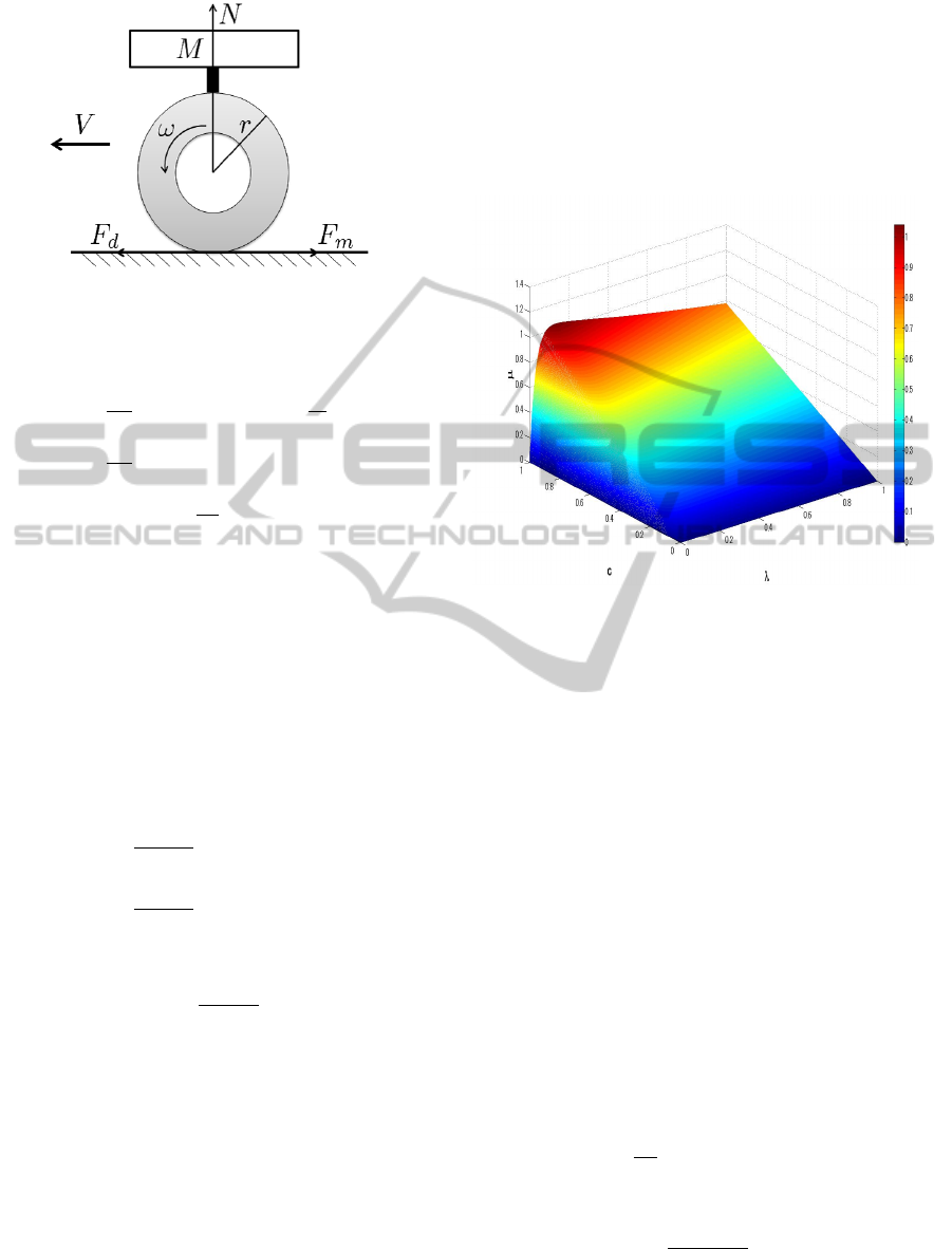
Figure 1: One-wheel car model.
From fig. 1, the vehicle dynamical equations are
expressed as eqs. (5) to (7).
M
dV
dt
= F
d
(λ) − F
a
−
T
r
r
(5)
J
dω
dt
= T
m
− rF
d
(λ) − T
r
(6)
F
m
=
T
m
r
(7)
F
d
= µ(c, λ)N (8)
Where M is the vehicle weight, V is the vehicle body
velocity, F
d
is the driving force, J is the wheel inertial
moment, F
a
is the resisting force from air resistance
and other factors on the vehicle body, T
r
is the fric-
tional force against the tire rotation, ω is the wheel
angular velocity, T
m
is the motor torque, F
m
is the
motor torque force conversion value, r is the wheel
radius, and λ is the slip ratio. The slip ratio is defined
by (9) from the wheel velocity (V
ω
) and vehicle body
velocity (V ).
λ =
V
ω
−V
V
ω
(accelerating)
V −V
ω
V
(braking)
(9)
λ during accelerating can be shown by (10) from fig.
1.
λ =
rω −V
rω
(10)
The frictional forces that are generated between
the road surface and the tires are the force generated
in the longitudinal direction of the tires and the lateral
force acting perpendicularly to the vehicle direction
of travel, and both of these are expressed as a func-
tion of λ. The frictional force generated in the tire
longitudinal direction is expressed as µ, and the re-
lationship between µ and λ is shown by (11) below,
which is a formula called the Magic-Formula(Pacejka
and Bakker, 1991) and which was approximated from
the data obtained from testing.
µ(λ) = −c
road
× 1.1 × (e
−35λ
− e
−0.35λ
) (11)
Where c
road
is the coefficient used to determine the
road condition and was found from testing to be ap-
proximately c
road
= 0.8 for general asphalt roads, ap-
proximately c
road
= 0.5 for general wet asphalt, and
approximately c
road
= 0.12 for icy roads. For the var-
ious road conditions (0 < c < 1), the µ − λ surface is
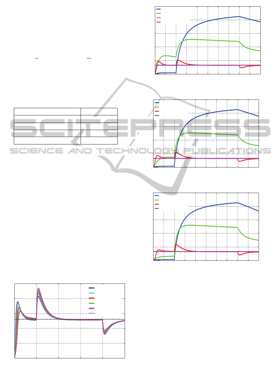
shown in fig. 2. It shows how the friction coefficient
Figure 2: λ-µ surface for road conditions.
µ increases with slip ratio λ (0.1 < λ < 0.2) where
it attains the maximum value of the friction coeffi-
cient. As defined in (8), the driving force also reaches
the maximum value corresponding to the friction co-
efficient. However, the friction coefficient decreases
to the minimum value where the wheel is completely
skidding. Therefore, to attain the maximum value of
driving force for slip suppression, it should be con-
trolled the optimal value of slip ratio. the optimal
value of λ is derived as follows.
Choose the function µ
c
(λ) defined as
µ
c
(λ) = −1.1 ×(e
−35λ
− e
−0.35λ
). (12)
By using (12), (11) can be rewritten as
µ(c,λ) = c
road
· µ
c
(λ). (13)
Evaluating the values of λ which maximize µ(c,λ)
for different c(c > 0), means to seek the value of λ
where the maximum value of the function µ
c
(λ) can
be obtained. Then let
d
dλ
µ
c
(λ) = 0 (14)
and solving equation (14) gives
λ =
log100
35 − 0.35
≈ 0.13. (15)
Thus, for the different road conditions, when λ ≈ 0.13
is satisfied, the maximum driving force can be gained.
SlidingModeSlipSuppressionControlofElectricVehicles
13

Namely, from (11) and fig. 2, we find that regardless
of the road condition (value of c), the λ − µ surface
attains the largest value of µ when λ is the optimal
value 0.13.
4 SMC METHOD WITH
INTEGRAL ACTION FOR SLIP
SUPPRESSION
In this section, for slip suppression of EVs, the pro-
posed control strategy based on SMC with introduc-
ing the integral term is explained. Without loss of
generality, one wheel model mentioned above is used
for design of the control laws. The system dynamics
can be written as
˙
λ = f + bT
m
(16)
where λ ∈ R is the state of system representing the
slip ratio of driven wheel which is defined as eq. (10)
for the case of acceleration. T
m
is the control input.
Differentiating eq. (10) with respect to time
˙
λ =
−
˙
V + (1 − λ)
˙
V
w
V
w
(17)
and substituting eqs. (5), (6) and (8) into eq. (17), the
following equations can be attained,
f = −
g
V
w
1 + (1 − λ)
r
2
M
J
w
µ(c,λ) (18)
b =
(1 − λ)r
J
w
V
w
. (19)
The control objective is to control the value of the
slip ratio to the constant reference value λ
∗
.
Actually, the mass of vehicle often changes with
the number of passengers and the weight of luggage.
Besides, the vehicle has to always travel on many
kinds of road surfaces. As a result, the controller
needs to perform much robustly with the uncertain-
ties happened in the mass of vehicle and road surface
conditions which are represented by M and c respec-
tively. The ranges of variation of M and c are set as
M
min
≤ M ≤ M
max
c
min
≤ c ≤ c
max
.
(20)
Consider the system eq. (16), the nonlinear func-
tion f is not exactly known, but it can be estimated as
ˆ
f . The estimation error on f is assumed to be bounded
by a known function F = F(λ),
ˆ
f − f
≤ F. (21)
The uncertainty in f is due to the parameter M and
c. Accordingly, by using eq. (18) the estimation of f
can be defined as
ˆ
f = −
g
V
w
1 + (1 − λ)
r
2
ˆ
M
J
w
µ( ˆc,λ)
(22)
where
ˆ
M is the estimated value of M and ˆc is esti-
mated for c.
Here, we define the estimated values of these pa-
rameters respectively by using the arithmetic mean of
the value of the bounds as
ˆ
M =
M
min
+ M
max
2
ˆc =
c
min
+ c
max
2
.
(23)
From these definitions, the error in estimation can
be given by
f −
ˆ
f
≤
g
|V
w
|
µ(c
max
,λ) − µ(ˆc,λ)
+(1−λ)
r
2
J
w
M
max
µ(c
max
,λ) −
ˆ
Mµ( ˆc,λ)
.(24)
Then, let
F =
g
|V
w
|
µ(c
max
,λ) − µ(ˆc, λ)
(1 − λ)
r
2
J
w
M
max
µ(c
max
,λ) −
ˆ
Mµ( ˆc,λ)
.(25)
4.1 Design of Sliding Surface
Letting
˜
λ be the variable of interest, then the order of
system is assumed to be one. The sliding function of
conventional SMC can be given by
s
c
(λ,t) =
˜
λ (26)
where
˜
λ is the error between the actual slip ratio and
the reference value, which is defined as
˜
λ = λ −λ
∗
.
By adding an integral item to the sliding function
s
c
, the new sliding function s can be designed as
s(λ,t) =
˜
λ + K
i
∫
t
0
˜
λ(τ)dτ (27)
where K
i
is the integral gain, K
i
> 0.
4.2 Derivation of Control Law
In this section, the sliding mode controller is derived
to make the slip ratio λ to track the reference slip ratio
λ
∗
. The sliding mode occurs when the state λ reaches
the sliding surface defined by s = 0. The dynamics of
sliding mode is governed by
˙s = 0. (28)
ICINCO2013-10thInternationalConferenceonInformaticsinControl,AutomationandRobotics
14

Differentiating eq. (27) and substituting the result
into eq. (28) give
˙
λ −
˙
λ
∗
+ K
i
λ − λ
∗
= 0. (29)
The reference slip ratio λ
∗
is a constant, thus
˙
λ
∗
=
0. Substituting eq. (16) into eq. (29) gives
f + bT
m
+ K
i
(λ − λ
∗
) = 0 (30)
and solving eq. (30) gives equivalent control input as
T
meq
=
1
b
− f − K
i
(λ − λ
∗
)
(31)
then the estimate of the equivalent control input can
be obtained as
ˆ
T
meq
=
1
b
−
ˆ
f − K
i
(λ − λ
∗
)
. (32)
For satisfying sliding condition (make state in the
sliding mode) despite uncertainty on the dynamics f ,
the hitting control input is defined as
T
mht
=
1
b
−Ksgn(s)
(33)
where
sgn(s) =
−1 s < 0
0 s = 0
1 s > 0
(34)
and K is called sliding gain. Thus, the control law can
be given by
T
m
=
ˆ
T
meq
+ T
mht
=
1
b
−
ˆ
f − K
i
(λ − λ
∗
) − Ksgn(s)
. (35)
When no uncertainty in the system (i.e., no varia-
tion in c and M), T
mht
is desired to be 0. Because eq.
(35) contains the estimate of the equivalent control
ˆ
T
meq
, T
m
keeps the state on the sliding surface (s = 0
i.e., λ = λ
∗
). Because of the uncertainties in the sys-
tem, the state λ could deviate from the sliding surface.
The hitting control acts to return the state back to the
sliding surface which implies the robustness of SMC.
Here, the sliding gain K is chosen as
K = F + η (36)
with the value of F given by eq. (25).
Then choose a Lyapunov function as
V =
1
2
s
2
(37)
and differentiate eq. (37) with respect to time, that
gives
˙
V =
1
2
d
dt
s
2
= s ˙s. (38)
Substituting eqs. (16), (28), (32), (33) and (35) into
eq. (38) yields
˙
V = s ˙s
= s
f −
ˆ
f − Ksgn(s)
= s( f −
ˆ
f ) − K|s|
≤ F|s| −K|s|
≤ −η|s|. (39)
Thus, the control law introduced in eq. (35) can
guarantee the stability of the system in the Lyapunov
sense under variations. Concretely, the stability of the
system is guaranteed with an exponential convergence
once the sliding surface is encountered, if the sliding
condition is satisfied. So eq. (39) guarantees the strat-
egy can converge to the sliding surface in finite time
if the error is not zero, that is to say, slip ratio can be
controlled to the reference value in finite time when-
ever the uncertainties occur in the system.
4.3 Chattering Reduction
For sliding mode control design, the switched con-
troller limits switching to a finite frequency, which
produces chattering. To reduce the chattering, the hit-
ting control T
mht
can be rewritten by using the satura-
tion function
T
mht
=
1
b
−Ksat
s
Φ
(40)
where Φ > 0 is a design parameter representing the
width of the boundary layer around the sliding surface
s = 0 and the saturation function is defined as
sat
s
Φ
=
−1 s < −Φ
s
Φ
−Φ ≤ s ≤ Φ
1 s > Φ
. (41)
Thus, using eqs. (35), (36) and (40), the control
law of the system by the proposed SMC can be rewrit-
ten as
T
m
=
1
b
−
ˆ
f −K
i
(λ− λ
∗
)−(F + η)sat
s
Φ
. (42)
5 NUMERICAL EXAMPLES
This section shows the numerical simulation results
to demonstrate the effectiveness of the proposed
method. In all simulations, we consider three dif-
ferent road conditions, a dry asphalt for t ∈ [0,2)[s],
an icy road for t ∈ [2, 8)[s] and a wet asphalt for
t ∈ [8,10][s]. The width of the boundary layer Φ de-
fied in eq. (40) is set to 1. In eq. (42), the proposed
SMC law can be calculated with the values of design
SlidingModeSlipSuppressionControlofElectricVehicles
15
parameters K
i
and η, which both impact on the steady
state accuracy. Here, for confirm the energy conserva-
tion performance of the proposed method, the values
of both parameters are set K
i
= 10 and η = 5, which
are determined by several tests.
By using eqs. (26), (28), (33) and (36), the control
law of the conventional SMC can be derived as
T
mc
=
1
b
−
ˆ
f − (F + η)sat
s
Φ
. (43)
In the conventional SMC, the parameters η = 1 and
Φ = 1. The value of parameters used in the simula-
tions are listed in Table 1.
Table 1: Parameters used in the simulations.
M:Mass of vehicle 1100[kg]
J
w
:Inertia of wheel 21.1[kg/m
2
]
r:Radius of wheel 0.26[m]
λ
∗
:Reference slip ratio 0.13
g:Acceleration of gravity 9.81[m/s
2
]
As the input to the simulation of system, the
torque is produced by the constant pressure on the ac-
celerator pedal, which is decided on the vehicle speed
desired by the driver. Here, the vehicle speed is de-
sired to achieve 180[km/h] in 15[s] by a fixed accel-
eration after starting the car. The range of variation
in mass of vehicle M and road condition coefficient
c are imposed as M
max
= 1400[kg], M
min
= 1000[kg],
c
max
= 0.9 and c
min
= 0.1 respectively. So the nomi-
nal values of mass and road condition coefficient can
be obtained as
ˆ
M = 1200[Kg] and ˆc = 0.5 .
5.1 Robust Performance
In order to verify the robustness of proposed SMC
with variation both in the mass of vehicle and road
condition, the variation in the mass of vehicle is made
0 2 4 6 8 10
0
0.05
0.1
0.15
0.2
0.25
Time (s)
Slip ratio
M=1000kg
M=1100kg
M=1200kg
M=1300kg
M=1400kg
reference value
Figure 3: Slip ratio by the proposed method.
0 1 2 3 4 5 6 7 8 9 10
0
0.2
0.4
0.6
0.8
1
Time (s)
Slip ratio
without control
with conventional SMC
with proposed SMC
reference value
Figure 4: Slip ratio (M = 1000[kg]).
0 1 2 3 4 5 6 7 8 9 10
0
0.2
0.4
0.6
0.8
1
Time (s)
Slip ratio
without control
with conventional SM
C
with proposed SMC
reference value
Figure 5: Slip ratio (M = 1200[kg]).
0 1 2 3 4 5 6 7 8 9 10
0
0.2
0.4
0.6
0.8
1
Time (s)
Slip ratio
without control
with conventional SMC
with proposed SMC
reference value
Figure 6: Slip ratio (M = 1400[kg]).
by assigning the value of M to 1000[kg], 1100[kg],
1200[kg], 1300[kg] and 1400[kg] respectively. Fig. 3
shows the responses of slip ratio with different masses
can converge to the reference value under the varia-
tion in the road condition. It is known that when the
mass gets the nominal value 1200[kg], in the first 2[s],
the response is more accurately than the car with other
mass. But after 2[s], the performance drops down with
the mass increases.
Next, we compared the proposed SMC with the
conventional SMC and no control. Figs. 4∼6 show
the responses of slip ratio under three different road
conditions for three different masses respectively.
ICINCO2013-10thInternationalConferenceonInformaticsinControl,AutomationandRobotics
16
The responses with proposed SMC can suppress
the slip ratio to the reference value 0.13 accurately in
a very short time whenever both of the mass and road
condition are changing. In addition, the slip ratio with
the conventional SMC does not converge to the refer-
ence value because of the steady state error. When the
car starts off at 0[s] or runs into an icy road at 2[s], the
slip ratio response using control method grows with
the increasing wheel speed as a result of too much
torque generated. As the car travels from icy road to
wet asphalt in 8[s], the slip ratio decreases with the
decreasing wheel speed, when the torque generated at
that time cannot satisfy the one required on the wet as-
phalt. The car without control is to make the slip ratio
to 0, so at the first stage the response is converged to
0. However, when the car runs into the ice road at 2
[
s
]
,
the wheel spins out of control resulting that the wheel
speed in-creasing suddenly, which leads to a large slip
ratio value. Therefore, we can see that the proposed
SMC has a good performance against the variation in
both of the mass of vehicle and road condition.
5.2 Acceleration Performance
It is different from the simulation condition described
in previous that the simulations are executed under
unchanging road condition with mass every time.
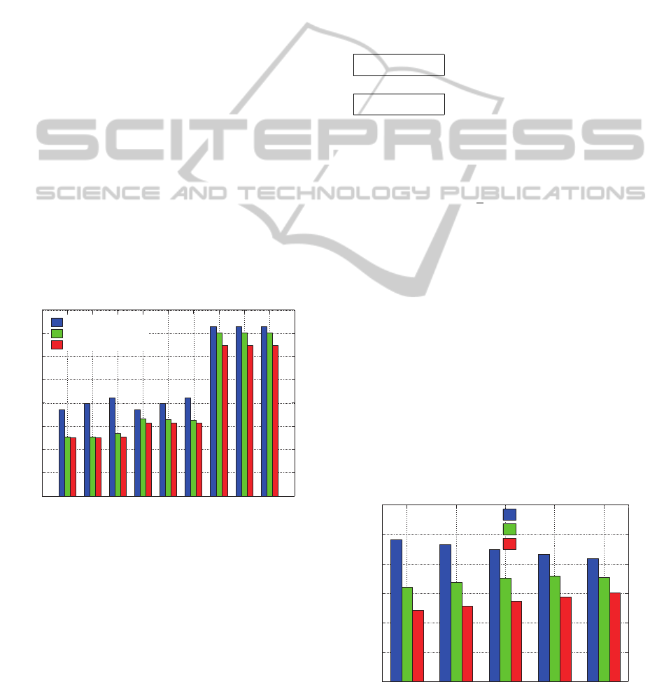
Figure 7: Acceleration performance.
Fig. 7 shows the time required for 100m by the car
with different control method. The x-axis label indi-
cates the cases of different road condition and mass,
for example, DA1000 says the car with M = 1000[kg]
is driving on the dry asphalt, WA1200 shows the case
with M = 1200[kg] on the wet asphalt and IR1400
is the case with M = 1400[kg] on the icy road. As
shown in fig. 7, it takes minimum time by the pro-
posed method in every case. So we can see that the
car with proposed SMC have gained the best accel-
eration. In other words, the results also indicate the
vehicle with the proposed SMC can keep the loss of
driving force at a minimum.
5.3 Energy Consumption
To confirm the effectiveness of the proposed SMC
for energy saving, we compare it to the conventional
SMC and no control method. Generally, It’s difficult
to evaluate the energy consumption accurately with-
out measurement by experiments on the real vehicle.
In this paper, therefore, we estimate the energy cost
by calculating the rotational energy of motor. As a
beginning, we give the following assumptions;
Assumption 1: the electric power is all used to
drive the wheel.
Assumption 2: the power consumed by the vehicle
is in proportional with the rotational energy due to
the rotation of driven wheel.
The rotational energy E
r
is defined by the rotational
inertia of wheel J
w
and the angular velocity w as
E
r
=
1
2
J
w
w
2
. (44)
Under these assumptions, we calculate the energy
consumed in the simulations in 5.1.
Fig. 8 shows the results of electric energy con-
sumed by different mass case. From this fig., we can
see that the proposed SMC consumes minimum en-
ergy in every case. The car without control takes most
energy because the spin of wheel on the icy road in
t ∈ [2,8)[s] leads to much energy loss. As the mass
increases, the amount of energy cost decreases be-
cause the car suppresses the spin of wheel by incre-
ment of mass to get more driving force. Conversely,
the energy consumption with the proposed SMC and
conventional SMC increases due to the rising cost of
control as the mass increases. From this perspective,
it also shows that an EV should be made more light to
save more energy.
M=1000kg M=1100kg M=1200kg M=1300kg M=1400kg
0
100
200
300
400
500
600
Electric energy consumed (Wh)
without control
with conventional SMC
with proposed SMC
Figure 8: Energy consumption.
SlidingModeSlipSuppressionControlofElectricVehicles
17

6 CONCLUSIONS
This paper proposes new SMC method with the in-
tegral action for EV traction control. The method
can improve the robust performance of EV traction
by controlling the slip ratio with low energy con-
sumption against the variation of mass of vehicle and
road conditions. We can verified that the the pro-
posed method shows good robust performance with
low energy consumption by comparing to conven-
tional method.
As future works, in this paper, the gain K
i
of in-
tegral action added in the sliding function was deter-
mined by trial and error, so it is necessary to develop
a systematic method to find the optimal value of K
i
.
Moreover, this paper was limited to showing the re-
sults with some example conditions using a simpli-
fied one wheel model, but to make the method practi-
cal, for a variety of road conditions and mass of vehi-
cle must be verified for more detailed two-wheel and
four-wheel models. In addition, the suitability of the
proposed method must be studied not only for the slip
suppression addressed by this paper but also for over-
all driving including during braking.
Even for this issue, however, the basic framework
of the proposed method can be used as is and can also
be extended relatively easily to form a foundation for
making practical high performed robust traction con-
trol systems with low energy consumption for EVs by
promoting further progress.
ACKNOWLEDGEMENTS
This research was partially supported by Grant-
in-Aid for Scientific Research (C) (Grant number:
24560538; Tohru Kawabe; 2012-2014) from the Min-
istry of Education, Culture, Sports, Science and Tech-
nology of Japan.
REFERENCES
Brown, S., Pyke, D. and Steenhof, P., 2010. Electric ve-
hicles: The role and importance of standards in an
emerging market, Energy Policy, Vol.38, Issue 7, pp.
3797–3806.
Mousazadeh, H., Keyhani, A., Mobli, H., Bardi, U., Lom-
bardi, G. and Asmar, T., 2009. Environmental assess-
ment of RAMseS multipurpose electric vehicle com-
pared to a conventional combustion engine vehicle,
Journal of Cleaner Production, Vol.17, Issue 9, pp.
781–790.
Hirota, T., Ueda, M. and Futami, T., 2011. Activities of
Electric Vehicls and Prospect for Future Mobility,
Journal of The Society of Instrument and Control En-
ginnering , Vol.50, pp. 165–170 (in Japanese).
Kondo, K., 2011. Technological Overview of Electric Ve-
hicle Traction, Journal of The Society of Instrument
and Control Enginnering (in Japanese), Vol.50, pp.
171–177.
Zanten, A. T., Erhardt, R. and Pfaff, G., 1995. VDC; The
Vehicle Dynamics Control System of Bosch, Proc. So-
ciety of Automotive Engineers International Congress
and Exposition 1995, Paper No. 950759.
Kin, K., Yano, O. and Urabe, H., 2001. Enhancements
in Vehicle Stability and Steerability with VSA, Proc.
JSME TRANSLOG 2001, pp.407–410 (in Japanese).
Sawase, K., Ushiroda, Y. and Miura, T., 2006. Left-Right
Torque Vectoring Technology as the Core of Super All
Wheel Control (S-AWC), Mitsubishi Motors Techni-
cal Review , No.18, pp.18–24 (in Japanese).
Kodama, K., Li, L. and Hori, H., 2004. Skid Prevention for
EVs based on the Emulation of Torque Characteristics
of Separately-wound DC Motor, Proc. The 8th IEEE
International Workshop on Advanced Motion Control
, VT-04-12, pp.75–80.
Mubin, M., Ouchi, S., Anabuki, M. and Hirata, H., 2006.
Drive Control of an Electric Vehicle by a Non-linear
Controller, IEEJ Transactions on Industry Applica-
tions , Vol.126, No.3, pp.300–308 (in Japanese).
Fujii, K. and Fujimoto, H., 2007. Slip ratio control based
on wheel control without detection of vehicle speed
for electric vehicle, IEEJ Technical Meeting Record,
VT-07-05, pp.27–32 (in Japanese).
Hori, Y., 2000. Simulation of MFC-Based Adhesion Con-
trol of 4WD Electric Vehicle, IEEJ Record of In-
dustrial Measurement and Control , IIC-00-12 (in
Japanese).
Kawabe, T., Kogure, Y., Nakamura, K., Morikawa, K. and
Arikawa, Y., 2011. Traction Control of Electric Vehi-
cle by Model Predictive PID Controller, Transaction
of JSME Series C, Vol. 77, No. 781, pp. 3375–3385
(in Japanese).
J. J. E. Slotine, J. J. E. and Li, W., 1991. Applied Nonlinear
Control, Prentice-Hall.
Eker, I., and AKinal, A., 2008. Sliding Mode Control with
Integral Augmented Sliding Surface: Design and Ex-
perimental Application to an Electromechanical sys-
tem, Electrical Engineering, Vol. 90, pp. 189–197.
H. B. Pacejka, H. B. and Bakker, E., 1991. The Magic For-
mula Tyre Model, Vehicle system dynamics, Vol.21,
pp.1–18.
ICINCO2013-10thInternationalConferenceonInformaticsinControl,AutomationandRobotics
18
