
Deriving the Conceptual Model of a Data Warehouse
from Information Requirements
Natalija Kozmina, Laila Niedrite and Maksims Golubs
Faculty of Computing, University of Latvia, Raina blvd. 19, Riga, Latvia
Keywords: Data Warehouse, Conceptual Model, Requirement Formalization, OLAP Schema Transformation.
Abstract: Business requirements are essential for developing any information system, including a data warehouse.
However, requirements written in natural language may be imprecise. This paper offers a model for
business requirement formalization according to certain peculiarities of elements of multidimensional
models, e.g. the distinction between quantifying and qualifying data. We also propose an algorithm that
generates candidate data warehouse schemas and is based on distinguishing data warehouse schema
elements in formal requirements. Then, resulting schemas are processed by a semi-automated procedure in
order to obtain a data warehouse schema that matches business requirements best of all.
1 INTRODUCTION
Companies should use performance measurement
systems, if they want to succeed in competition with
others. During the performance measurement, its
results should be compared with the target values to
understand, whether goals are achieved or not. For
implementation of a performance measurement
system a data warehouse could be used.
"A data warehouse is a subject-oriented,
integrated, non-volatile, and time-variant collection
of data in support of management decisions"
(Inmon, 2002). Developing a data warehouse that
fits all requirements of potential users is not the
easiest task. There is no common understanding
about the best method for conceptual modeling of
data warehouses and the most expressive modeling
language for that purpose. Conceptual models of
data warehouses can be classified according to their
origination (Rizzi et al., 2006): E/R model based,
UML based, and independent conceptual models,
e.g. Dimensional Fact Model (Golfarelli et al.,
1998). The necessity to develop special conceptual
models for data warehouses is founded on existence
of two types of data that should be modeled –
quantifying and qualifying data, and elements of
multidimensional paradigm, e.g. dimensions,
hierarchies, cubes, whose semantics can’t be
modeled properly with standard modeling
languages. Besides the specialized conceptual
models for data warehouses, developers also need
formal methods to construct these models (Rizzi,
2009). All methods can be classified as supply- or
demand-driven according to the way how the data
warehouse requirements are determined. The
requirements for data warehouses differ from those
applied to other types of systems – here we can
speak about the information requirements (Winter
and Strauch, 2003). In supply-driven methods the
existing models of data sources are investigated to
understand what data is used in an enterprise. In
demand-driven approaches the required data for
analysis needs is established mostly by interviewing
users. However, more new approaches, e.g.
ontology-based (Romero and Abello, 2010), pattern-
based (Jones and Song, 2005), are proposed to gain
the most suitable conceptual model of a data
warehouse for the implementation of the strategy of
an organization and to avoid the limitations of
existing methods. In the supply-driven approach the
constructed conceptual model may not reflect all
analysis needs, because it reflects the operational
needs of data source systems. In the requirement-
driven approach the data warehouse model depends
on interviewed users, their understanding about the
enterprise, and ability to precisely express their
analysis needs.
We propose a method for transforming
information requirements to conceptual model of a
data warehouse. In this case, requirements are
136
Kozmina N., Niedrite L. and Golubs M..
Deriving the Conceptual Model of a Data Warehouse from Information Requirements.
DOI: 10.5220/0004426301360144
In Proceedings of the 15th International Conference on Enterprise Information Systems (ICEIS-2013), pages 136-144
ISBN: 978-989-8565-59-4
Copyright
c
2013 SCITEPRESS (Science and Technology Publications, Lda.)

performance indicators of an organization that are
gathered by interviewing users and formalized in
accordance with the indicators model.
The rest of the paper is organized as follows.
Section 2 describes related work. Section 3
introduces formal model for indicator definition.
Section 4 presents the algorithm that transforms
requirements. Section 5 describes the post-
processing of schemas produced by algorithm.
Section 6 ends the paper with conclusions.
2 RELATED WORK
Demand-driven methods can be divided more
precisely according to the way of identifying
requirements, e.g. user-driven (Westerman, 2001),
(Poe, 1996) process-driven (Kaldeich and Oliveira,
2004), and goal-driven (Giorgini et al., 2005), (List
and Machaczek, 2004) where users are interviewed
and processes, goals, or indicators are modeled and
analyzed to gain precise understanding of analysis
needs of users and the organization. For example,
(Poe, 1996) proposes a catalogue for storage of
users’ interviews to collect end-users’ requirements,
recommends to interview different groups of users
to understand a business completely. In case of the
process-driven approach, a business process is
analyzed, e. g., in (Kaldeich and Oliveira, 2004) the
“AS IS” and “TO BE” process models are
constructed including the analyzed processes, as
well as the corresponding data models. In case of
the goal-driven approach, goals of an enterprise,
goals of analyzed business processes are analyzed
and data that should be analyzed to achieve these
goals is identified. For example, in (Giorgini et al.,
2005) the decisional modeling is performed, facts
are identified and mapped onto entities or relations
of data sources, but hierarchies of each fact are later
constructed by applying supply-driven approach
(Golfarelli et al., 1998).
In information supply-driven approach we can
speak about methods e.g. (Inmon, 2002), (Golfarelli
et al., 1998) that utilize the existing data models of
transaction systems. A data warehouse model is
obtained by transforming models of data sources.
For example, (Golfarelli et al., 1998) analyze many-
to-one associations in the data source models to
construct an attribute tree that is used later to form
dimensions, hierarchies, and other elements of
multidimensional paradigm.
3 THE FORMAL MODEL
FOR INDICATOR DEFINITION
Data warehouses have specific features when they
are used for implementation of performance
measurement systems: new data sources, e.g.
workflow logs, specific data analysis approaches,
e.g. process monitoring based on performance
indicators, and data warehouse model that reflects
the previous two aspects, which may determine the
data items to be included into the data warehouse
model.
Indicators are the focus of data analysis in the
performance measurement process. The definition
of indicators can be expressed on various levels of
formality. We proposed a formal specification of
indicators in our previous work (Niedritis et al.,
2011). At the same time, the data warehousing
models are built to represent the information needs
for data analysis. So, we could perceive indicators
as an information requirement for a data warehouse
system. Therefore, the formalization of indicators
could be based on the nature of elements of
multidimensional models, e.g. the distinction
between quantifying and qualifying data.
The type of an information system to be
developed has some impact on the way of
formulating sentences that express requirements.
Before starting our study, we assumed that
information requirements for data warehouses used
for performance measurement have similar
structure. This assumption was based on our
observations on how the information needs were
described in real life projects. We based the
proposed model also on the structure evaluation of
the sentences that formulate performance indicators
taken from the performance measures database
(Parmenter, 2010).
3.1 Concepts of the Formal Model
of Requirements
The requirement formalization is represented as a
UML class diagram by (Niedritis et al., 2011).
show Refinement Action
month Qualifiyng Data
AVG Aggregation Action
contacts ocurrance Quantifying Data
where
customer type Qualifiyng Data Simple Expression
=
'key customer' Constant Simp le Expression
Simple Requirement
Condition Type
Operation
Operation
Object
Object
Comparison
Simple
Condition
Typified
Condition
Figure 1: Requirement formalization example (Niedritis et
al., 2011).
DerivingtheConceptualModelofaDataWarehousefromInformationRequirements
137

In this paper we use an implementation model of
the requirements formalization for the algorithm
described in Section 4.2, but for better
understanding we give a short description of main
concepts in this section.
Let’s see an indicator example: “Average
number of contacts made with key customers per
month”. Using our proposed requirement model it is
reformulated as follows: “show month, average
(contact occurrence) where customer type is ‘key
customer’ ”. Figure 1 demonstrates the application
of the model. The left column is filled with parts of
the requirement statement and all the rest columns
(left to right) contain names of the model levels.
In the proposed model a requirement can be
classified as Simple or Complex Requirement. A
complex requirement is composed of two or more
simple requirements with an Arithmetical Operator.
A simple requirement consists of a verb (Operation)
that denotes a command, which refers to an Object,
and zero or one Typified Condition. There are two
kinds of data in data warehousing: Quantifying
(measurements) and Qualifying (properties of
measurements). An object is either an instance of
quantifying or qualifying data depending on the
requirement.
A Complex Operation consists of two or more
Actions. There are two possible types of action:
Aggregation (used for calculation and grouping,
“roll-up”) and Refinement (used for information
selection, “drill-down”, as an opposite to an
aggregation). Information refinement is either
showing details, i.e., selecting information about
one or more objects, or slicing, i.e., showing details,
according to a certain constraint (Typified
Condition). Conditions can be simple or complex.
Complex condition joins two or more simple
conditions by Logical Operators (AND, OR, NOT).
Simple condition consists of a Comparison of two
Expressions, for example, “time is greater than
last_access_time – 1 second”. An expression too
may be either a Simple or a Complex Expression. A
complex expression contains two or more simple
expressions with an arithmetical operator between
the simple expressions. A simple expression belongs
either to qualifying data (e.g. “last_access_time”) or
to Constants (e.g. “1 second”).
3.2 The Implementation Model
of Formal Requirements
Formal requirement metadata is implemented using
relational database tables depicted in Figure 2.
Requirements are stored in tables Requirement and
SimpleRequirement. Each business requirement
refers to some theme (Theme), e.g. Finance,
Customer Focus, etc. Simple requirements are
defined by Operation, Object and
TypifiedCondition. An operation is either an
aggregate function (isAggr=1) or a refinement
operation (isAggr=0). An operation can consist of
multiple suboperations, e.g. SUM(AVG(Income)).
To indicate the sequence of them, an attribute
Operation.Index is employed. The value of
Object.Type is either ‘qualifying’ or ‘quantifying’.
A simple condition involves two expressions and
the value of a comparison. The expression type is
defined by Expression.isSimple. A simple
expression consists of either a qualifying data
object, or a constant, and the type of an expression
(Expression.Type) respectively. Otherwise, an
expression is composed of multiple expressions and
an arithmetical (Expression.ArithmeticalOperator)
operator between them. A complex condition
involves conditions and a logical operator.
Requirement
PK ID
isSimple
FK1 Requirement1ID
FK2 Requirement2ID
ArithmeticalOperator
Index
FK3 SimpleReqID
FK4 ThemeID
SimpleRequirement
PK ID
FK1 ObjectID
FK2 TypifiedConditionID
FK3 OperationID
Object
PK ID
Name
Type
isTime
Operation
PK ID
isAggr
Value
Index
SuboperationID
TypifiedCondition
PK ID
Value
FK1 ConditionID
Condition
PK ID
isSimple
FK1 Condition1ID
FK2 Condition2ID
LogicalOperator
Comparison
FK3 Expression1ID
FK4 Expression2ID
Expression
PK ID
isSimple
Type
Constant
FK1 Expression1ID
FK2 Expression2ID
ArithmeticalOperator
FK3 ObjectID
Theme
PK ID
Name
Figure 2: The implementation model of formal
requirements.
4 FROM REQUIREMENTS
TO PRE-SCHEMAS
In this paper we propose a method for transforming
information requirements to the conceptual model of
a data warehouse (see Figure 3). The method uses
requirements from formal requirements database
and generates a simplified data warehouse schema
(pre-schema or candidate schema) by an algorithm
that analyses the structure of requirements. The next
stage of the method is semi-automated candidate
schemas are processed and restructured to remove
ICEIS2013-15thInternationalConferenceonEnterpriseInformationSystems
138

duplicates and build dimension hierarchies. Finally,
the improved schemas can be used as data
warehouse schema metadata.
Formal requirements
implementation
model
Pre-schema
Pre-schema Generation
Algorithm
Semi-automated execution
Data warehouse
model
Copy restructured
pre-schema
Pre-schema restructuring component
Figure 3: Pre-schema generation and restructuring.
4.1 A Pre-Schema and its Components
When exploring formal requirements, measures
(C_Measure) that characterize business processes
are determined and so do attributes (C_Attribute)
that describe measures. PreSchema is a candidate
schema of a data warehouse that includes measures
and attributes derived from requirements. In Figure
4 an implementation model for storing candidate
schemas and its elements is depicted.
PreSchema
PK ID
FK1 ThemeID
Index
isAccepted
C_Measure
PK ID
FK1 PreSchemaID
Name
DataType
isAccepted
Theme
PK ID
Name
C_Attribute
PK ID
Name
FK1 PreSchemaID
isTime
isAccepted
C_Aggregation
PK ID
FK1 MeasureID
Value
isAccepted
Index
C_Level
ID
FK1 AttributeID
Name
C_Hierarchy
PK ID
Name
C_LevelHierarchy
ID
FK1 HierarchyID
FK2 LevelID
Index
C_AcceptableAggregation
PK ID
FK1 AttributeID
FK2 AggregationID
isAccepted
Figure 4: A candidate schema (PreSchema) and its
components.
PreSchema.Index represents a link to a simple
requirement in requirement model. If in a formal
requirement a measure has an aggregate function
applied to it, then it is stored in C_Aggregation.
Tables C_Level, C_Hierarchy and
C_LevelHierarchy are employed to define attribute
hierarchies. C_LevelHierarchy.Index is some level’s
sequence number in a hierarchy. The meaning of an
attribute isAccepted in PreSchema, C_Measure,
C_Attribute, C_Aggregation, and
C_AcceptableAggregation is described in Section 5.
4.2 PGA: The Pre-Schema Generation
Algorithm
We propose a pre-schema generation algorithm
(PGA) for distinguishing data warehouse pre-
schema elements in formal requirements stored in an
implementation model (see Figure 2).
In Procedure 1 (MakePreSchema) requirements
are reviewed in a context of the business
requirement theme (lines 1-3). All simple
requirements of a certain theme are processed (lines
4-22). Complex requirements are not reviewed,
because objects, operations, and conditions are
defined in simple requirements only.
If the type of an object is Quantifying, then it is a
measure – C_Measure (lines 11-13). To find
aggregate functions (C_Aggregation) associated
with the measure and to set its order, operations are
checked by Function 1 (ProcessOperations; line 14,
and 23-40). If the type of an object is Qualifying,
then it is processed as an attribute – C_Attribute
(lines 15-18). Finally, simple conditions are handled
by Procedure 2 (ProcessSimpleConditions; line 22,
and 41-54). If an expression in a simple condition
has the type Qualifying, then the appropriate object
is an attribute (lines 46-51). Expressions with the
type Constant are ignored.
5 THE PROCESSING
OF A PRE-SCHEMA
Before discussing the process model of handling
pre-schemas generated by PGA, the following
assumptions should be considered:
Two measures in a set of pre-schemas have the
same name, iff their semantic meaning is the same.
For instance, if two measures are named “total
number”, however, semantically one of them
corresponds to “total number of students” and the
other one – to “total number of teachers”, then
these two measures should be renamed
respectively.
Two attributes in a set of pre-schemas have the
same name, iff their semantic meaning is the same.
The explanation is equivalent to the above-
mentioned, but is related to attributes.
Names of the measures in pre-schemas coincide
with those in the data source.
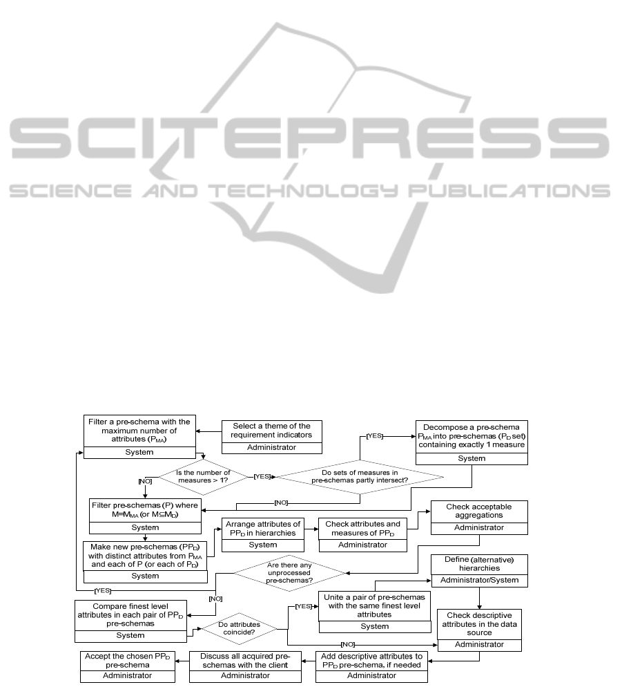
First of all, an administrator picks up a certain
theme to which a set of pre-schemas gained from
requirements refers. Then, a pre-schema with the
maximum number of attributes is selected. Let us
call such pre-schema P
MA
. If there are multiple P
MA
-
like pre-schemas with different sets of attributes,
their processing goes independently and is just the
same as the one of P
MA
pre-schema. In Figure 5 we
DerivingtheConceptualModelofaDataWarehousefromInformationRequirements
139

PGA Procedure 1: MakePreSchema, Input: CurrentTheme:Theme
1: IF NOT EXIST Theme WHERE Theme.Name = CurrentTheme.Name
2: THEN (CREATE Theme; Theme.Name:=CurrentTheme.Name;)
3: ELSE FIND Theme WHERE Theme.Name = CurrentTheme.Name;
4: FOR EACH Requirement WHERE Requirement.isSimple = 1
5: AND Requirement.ThemeID = CurrentTheme.ID DO:
6: CREATE PreSchema; PreSchema.Index:=Requirement.Index;
7: PreSchema.ThemeID:=Theme.ID;
8: FIND SimpleRequirement
9: WHERE SimpleRequirement.ID = Requirement.SimpleReqID;
10: FIND Object WHERE Object.ID = SimpleRequirement.ObjectID;
11: IF Object.type = 'Quantifying' THEN (
12: CREATE C_Measure; C_Measure.PreSchema:=PreSchema.ID;
13: C_Measure.Name:=Object.Name;
14: ProcessOperations(SimpleRequirement.OperationID, C_Measure.ID);)
15: ELSE (
16: CREATE C_Attribute; C_Attribute.PreSchemaID:=PreSchema.ID;
17: C_Attribute.Name:=Object.Name;
18: C_Attribute.isTime:=Object.isTime;)
19: FIND TypifiedCondition WHERE
20: TypifiedCondition.ID = SimpleRequirement.TypifiedConditionID;
21: FIND Condition WHERE Condition.ID = TypifiedCondition.ConditionID;
22: RUN ProcessSimpleConditions(Condition.ID, PreSchema); END.
PGA Function 1: ProcessOperations, Input: CurrID:number, CurrMeasureID:number
23: FIND Operation WHERE Operation.ID = CurrID;
24: IF Operation.SuboperationID != NULL
25: THEN (OperationIndex:=ProcessOperations(Operation.SuboperationID, CurrMeasure);
26: IF Operation isAggr = 1 THEN (CREATE C_Aggregation;
27: FIND C_Measure WHERE Measure.ID = CurrMeasure;
28: C_Aggregation.MeasureID:=C_Measure.ID;
29: C_Aggregation.Value:=Operation.Value;
30: C_Aggregation.Index:=(OperationIndex + 1);
31: RETURN OperationIndex + 1.)
32: ELSE
33: RETURN OperationIndex.)
34: ELSE (
35: IF Operation isAggr = 1 THEN (CREATE C_Aggregation;
36: FIND C_Measure WHERE Measure.ID = CurrMeasure;
37: C_Aggregation.MeasureID:=C_Measure.ID;
38: C_Aggregation.Value:=Operation.Value;
39: C_Aggregation.Index:=1;
40: RETURN 1.))
PGA Procedure 2: ProcessSimpleConditions, Input: CurrentConditionID:number, CurrentPreSchema:PreSchema
41: FIND Condition WHERE Condition.ID = CurrentConditionID;
42: IF Condition.isSimple = 1 THEN (
43: FOR EACH Expression
44: WHERE Expression.ID = Condition.Expression1ID
45: OR Expression.ID = Condition.Expression2ID DO:
46: IF Expression.Type = 'Qualifying' THEN (
47: FIND Object WHERE Object.ID = Expression.ObjectID;
48: CREATE C_Attribute;
49: C_Attribute.PreSchemaID:=CurrentPreSchema.ID;
50: C_Attribute.Name:=Object.Name;
51: C_Attribute.isTime:=Object.isTime;) END.
52: ELSE (
53: ProcessSimpleConditions(CurrentCondition.Condition1ID, CurrentPreSchema);
54: ProcessSimpleConditions(CurrentCondition.Condition2ID, CurrentPreSchema);) END.
ICEIS2013-15thInternationalConferenceonEnterpriseInformationSystems
140
ignored the case of multiple pre-schemas with the
same maximum number of attributes on purpose for
better understanding.
A pre-schema may contain a set of measures
(M1, M2 …, Mn). Further manipulations with the
pre-schema depend on the number of measures that
it contains. Having more than one measure, certain
rules take place:
1. If there is at least one pre-schema with a set of
measures that in any way intersects with a
measure or a set of measure of another pre-
schema (e.g. (M1, M2) ∩ (M2, M3, M4) = M2;
(M1, M2) ∩ M1 = M1, etc.), then all pre-schemas
with intersecting measures should be
decomposed, because the meaning and
granularity of fact measures are determined by
the finest level attributes.
2. If the set of all pre-schemas contains different
sets of measures (e.g. (M1, M2); (M3, M4, M5);
M6; M7; etc.) that do not have overlapping
elements, then there is no need to decompose the
pre-schemas.
3. If a set of measures is the same for all pre-
schemas assigned to a certain theme, then none of
the pre-schemas should be decomposed.
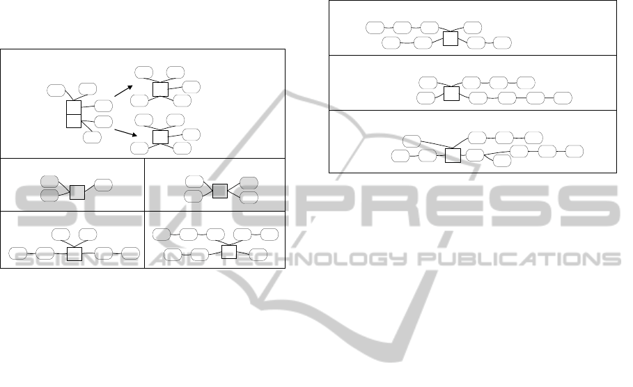
In case of (1), a pre-schema P
MA
is being
decomposed into pre-schemas each of which
contains only one measure, and a set of attributes is
equal to that of P
MA
. An example of decomposing a
pre-schema with two measures is depicted in Figure
6a. Let’s call each of the newly acquired pre-
schemas in Figure 6a P'
D
and P''
D
.
Pre-schemas that contain the same measure as
P
MA
(or at least one of the decomposed pre-
schemas) are of interest. Let’s call a set of filtered
pre-schemas P. Examples of such pre-schemas are
illustrated in Figure 6 (b – pre-schema P', and c –
pre-schema P'') containing two different measures:
M1 as in P'
D
, M2 as in P''
D
.
PP'
D
and PP''
D
are new pre-schemas that consist
of measures and attributes from P'
D
and P''
D
respectively, and attributes that exist in each of pre-
schemas of set P but are missing in the pre-schema
P'
D
(in Figure 6b – attribute A6) and P''
D
(in Figure
6c – attributes A7, A8, and A9). However, before
the attributes are actually added to either PP'
D
or
PP''
D
, they should be arranged in hierarchies, so that
measures would be described by the finest level
attributes only. In Figure 6d PP'
D
is an example of
arranging distinct attributes from P'
D
and P', whereas
in Figure 6e PP''
D
is the example of arranging those
from P''
D
and P''.
To order attributes of pre-schemas in hierarchies,
we follow some data-driven algorithm (e.g.
(Golfarelli et al., 1998)). First, an arbitrary attribute
(let’s denote it as A) from a set of distinct attributes
of, say, P'
D
and P' is selected. Then, in the data
source a certain entity attribute (let’s denote it as
M
E
) that corresponds to the measure of a pre-
schema P'
D
is determined.
Next, we move from M
E
to all attributes that
have a many-to-one relationship with M
E
. We
traverse in such way the attributes in data source
until an attribute that corresponds to A is found
(A
E
). When found, A is classified either as a finest
hierarchy level (if M
E
is connected to A
E
directly) or
a coarser hierarchy level (if M
E
is connected to A
E
through two or more M:1 associations) of a certain
hierarchy of the pre-schema PP'
D
.
Figure 5: The process model of handling pre-schemas generated by PGA.
DerivingtheConceptualModelofaDataWarehousefromInformationRequirements
141
All attributes that can be reached from A
E
by
M:1 association and do exist in pre-schema PP'
D
are
ordered in hierarchy the same way as they have
been traversed in the data source – from finest to
coarsest level. Finally, the property isAccepted of all
processed attributes and measures in the pre-schema
PP'
D
that have a matching entity attribute in the data
source are updated to 1.
(a) P
MA
P'
D
A1
A2
A3
A4
A5
M1
M2
A1 A2
A3
A4A5
M1
A1 A2
A3
A4A5
M2
P''
D
(b) P'
A1
A5
A6
M1
(c) P''
A7
A8
A2
M2
A9
(d) PP'
D
A1
A2
A3
A4
A5
M1
A6
(e) PP''
D
A1
A2
A3
A4
A5
M2
A8 A7A9
Figure 6 a: A pre-schema with maximum attribute count
(P
MA
) is being decomposed into two pre-schemas (P'
D
and
P''
D
); b, c: two pre-schemas (P' and P''); d, e: PP'
D
and
PP''
D
: pre-schemas P'
D
and
P''
D
supplemented with
attributes from P' and P'' respectively, ordered in
hierarchies.
If an attribute or a measure exists only in
requirements (i.e., in pre-schemas), then the
property isAccepted of the attribute or measure is
updated to 0. Also, it may happen that A
E
cannot be
reached from M
E
by M:1 associations. Then A has
the property isAccepted updated to 0 too. Such
attributes or measures will be reviewed by
administrator later on. Also, an administrator should
review all aggregate functions that are applied to
additive, semi-additive or non-additive measures to
either accept an aggregation if its application to a
certain measure is allowed, or decline if its
application to the measure is inappropriate. The
property isAccepted of the C_Aggregation and
C_AcceptableAggregation is modified in obedience
to the measure type. By that we indicate that certain
elements of the modified P
MA
(or P'
MA
) pre-schema
are ready for further analysis.
If there are any pre-schemas with measures that
differ from those in already processed pre-schemas,
then the algorithm is being iteratively executed from
the step where a pre-schema with the maximum
attribute count is found.
The next step of the process is aimed at making
a union of two or more pre-schemas on condition
that all finest hierarchy level attributes coincide. If
this condition isn’t satisfied, then this step should be
skipped.
(a)
A1 A2
A4 A12A5
M
A8
A7
A9
(b)
A2
A5 A4 A11
A1
A6
M
A10
A8 A9
(c)
A2
A5
A4
A11
A1
A6
M
A10
A8 A9
A12
A7
Figure 7 a, b: An example of hierarchies in two different
pre-schemas with the same finest hierarchy level
attributes and same measures; c: an example of the union
of two pre-schemas.
Consider an example in Figure 7: there are two pre-
schemas with the same finest hierarchy level
attributes and same measures, however, coarser
hierarchy level attributes might differ. Hierarchies
in Figure 7a are: H1a: A5A7; H2a: A1A8A9;
H3a: A2; H4a: A4A12. Hierarchies in in Figure
7b are: H1b: A5; H2b: A2; H3b: A1A8A9;
H4b: A4A6A10A11. It is possible to unite
two (or more) pre-schemas, taking into an account
several rules:
If two hierarchies are equivalent (H2a ≡ H3b, H3a
≡ H2b), then one of the equivalent hierarchies will
be added with no changes to the united pre-
schema.
If finest hierarchy level attributes are similar, but
coarser hierarchy level attributes differ, then all
alternative hierarchies will be included in the
united pre-schema (both H4a and H4b).
If finest hierarchy level attributes are similar, but
in some hierarchies coarser level attributes are
absent, then the hierarchy with the largest number
of levels will be added to the united pre-schema
(only H1a).
As a result, there is a pre-schema with the
following hierarchies: A5A7; A1A8A9; A2;
A4A12; A4A6A10A11 (see Figure 7c).
Data source attributes may be divided into two
groups: the ones that are equivalent to the attributes
in pre-schemas gained from requirements, and the
ones that aren’t. Let’s call the latter descriptive
attributes as they might provide additional
information on the attributes in pre-schemas. An
ICEIS2013-15thInternationalConferenceonEnterpriseInformationSystems
142

administrator may add descriptive attributes to pre-
schemas, if it is necessary.
The last step but one is an interview with the
client during which all generated pre-schemas are
being shown. The client should make a decision and
choose one pre-schema that would meet the
requirements for a new schema best of all.
Finally, to indicate that one of the pre-schemas
is selected, an administrator updates the isAccepted
property of a pre-schema to 1, and the pre-schema is
being copied to the data warehouse metadata
repository that mostly complies with CWM
(Solodovnikova, 2008).
6 CONCLUSIONS
In this paper we set forth an approach of building a
candidate schema (pre-schema) of a data warehouse
that complies with the business requirements stated
by the client. We consider requirements as
performance indicators of an organization that are
gathered during the interview and formalized in
accordance with the indicators model described in
detail in (Niedritis et al., 2011).
The contribution of this paper is the pre-schema
generation algorithm (PGA) that employs
indicators, and the description of the semi-
automated pre-schema post-processing. We believe
that pre-schemas acquired this way will be more apt
then schemas gained by applying other demand-
driven methods. During the post-processing, pre-
schema hierarchies are defined by a data-driven
algorithm. However, there certainly are some
presumptions that should be fulfilled first to enable
the usage of PGA; for instance, (i) requirements
have to be formalized in a specific way, (ii)
measures or attributes with the same name but
different semantic meaning should be renamed to be
distinguishable from one another.
Our future work would include the
implementation of the PGA, its testing on a large set
of indicators of an existing data warehouse schemas
followed by its evaluation. Also, quality attributes
for evaluations of accepted pre-schemas should be
introduced. Afterwards, the pre-schemas defined by
PGA would be processed and the resulting pre-
schema(s) would be compared with the existing data
warehouse schemas.
ACKNOWLEDGEMENTS
This work has been supported by ESF project
No.2009/0216/1DP/1.1.1.2.0/09/APIA/VIAA/044.
REFERENCES
Giorgini P., Rizzi S., Garzetti M. 2005. Goal-oriented
requirement analysis for data warehouse design. In:
Proc. of 8th ACM Int. workshop on Data
Warehousing and OLAP (DOLAP'05), ACM Press,
New York, pp 47-56
Golfarelli M., Maio D., Rizzi S. 1998. Conceptual design
of data warehouses from E/R schemes. In: Proc. of
31st Annual Hawaii Int. Conf. on System Sciences
(HICSS'98), Kona, Hawaii, IEEE, USA, 7:334-343
Inmon W.H. 2002. Building the data warehouse. 3rd edn.,
Wiley Computer Publishing
Jones M. E., Song I. 2005. Dimensional modeling:
identifying, classifying and applying patterns. In:
Proc. of 8th ACM Int. workshop on Data
Warehousing and OLAP (DOLAP'05), ACM Press,
New York, pp 29-38
Kaldeich C., Oliveira J. 2004. Data warehouse
methodology: a process driven approach. LNCS 3084.
Springer, Heidelberg, pp 536-549
List B., Machaczek K. 2004. Towards a corporate
Performance Measurement System. In: Proc. of ACM
symposium on Applied Computing (SAC'04), ACM
Press, New York, pp 1344-1350
Niedritis, A., Niedrite, L., Kozmina, N. 2011.
Performance Measurement Framework with Formal
Indicator Definitions. In: Grabis, J., Kirikova, M.
(eds.) BIR 2011. Springer, Heidelberg, LNBIP, 90:44-
58
Parmenter D. 2010. Key Performance Indicators:
developing, implementing, and using winning KPIs.
2nd edn., Jon Wiley & Sons, Inc.
Poe V. 1996. Building a data warehouse for decision
support. Prentice Hall
Rizzi S. 2009. Conceptual Modeling Solutions for the
Data Warehouse. In: Erickson, J. (ed.) Database
Technologies: Concepts, Methodologies, Tools, and
Applications, IGI Global, pp 86-104
Rizzi S., Abelló A., Lechtenbörger J., Trujillo J. 2006.
Research in data warehouse modeling and design:
dead or alive? In: Proc. of 9th ACM Int. workshop on
Data Warehousing and OLAP (DOLAP'06), ACM
Press, New York, pp 3-10
Romero O., Abello A. 2010. A framework for
multidimensional design of data warehouses from
ontologies. Data and Knowledge Engineering
69:1138-1157
Solodovnikova, D. 2008. Metadata to support data
warehouse evolution. In: Proc. of 17th Int. Conf. on
Information Systems Development (ISD'08), Paphos,
Cyprus, 2008, pp 627-635
DerivingtheConceptualModelofaDataWarehousefromInformationRequirements
143

Westerman P. 2001. Data warehousing using the Wal-
Mart model. Morgan Kaufmann
Winter R., Strauch B. 2003. A method for demand-driven
information requirements analysis in data
warehousing projects. In: Proc. of 36th Annual
Hawaii Int. Conf. on System Sciences (HICSS'03),
Waikoloa, Hawaii, IEEE, USA, pp 1359-1365
ICEIS2013-15thInternationalConferenceonEnterpriseInformationSystems
144
