
Mobile Robot Localization based on a Set Approach using
Heterogeneous Measurements
Etienne Colle, Simon Galerne and Maxime Jubert
IBISC, University Of Evry, Evry, France
Keywords: Robot Mobile Localization, Interval Analysis, Inversion Set, Heterogeneous Measurements Fusion,
Cooperative Environment.
Abstract: This work tackles the problem of the localization of a robot in in large and cooperative environments using
real-time data coming either from the robot onboard sensors or/and from the sensors in the environment.
The paper focuses on the 3-DOF localization of a mobile robot that is to say the estimation of the robot
coordinates (xmr, ymr, θmr) in a 2D-environment. The problem of nonlinear bounded-error estimation is
viewed as a set inversion. The paper presents the theoretical formulation of the localization method in a
bounded-error context and the parameter estimation based on interval analysis. Simulation results as well as
real experiments show the contributions of the method. The method is able to easily integrate a large variety
of sensors, from the roughest to the most complex one. The method takes into account a heterogeneous set
of measurements, a flexible number of measurements, a statistical knowledge on the measurements limited
to the tolerance, and the fact the measurements are acquired both from the robot onboard sensors and the
environment sensors. The way that environment model inaccuracies can be taken into account is also
presented.
1 INTRODUCTION
The ability of a mobile robot to perform various
home services for human beings in cluttered or
dynamically changing environment requires a
reliable robot localization. In the context of the
ubiquitous robotics many studies have attempted to
improve the accuracy and the reliability of robot
localization using the redundancy given by a sensor
network. Works are divided into three approaches:
localization based on homogeneous sensor network,
localization based on hybrid sensor networks and
localization based on sensor networks and onboard
robot sensors. (Zhang et al., 2007) exploited a
distributed and homogeneous sensor network using
infrared sensors. The infrared sensors were
suspended from the ceiling. (Han et al., 2007)
proposed a localization system for mobile agents
using passive RFID tags that were arranged on the
floor of an indoor space. Others authors as (Shenoy
and Tan, 2005) addressed the localization algorithm
with a hybrid sensor network. For accurate
localization the existing research might fuse sensor
networks and general sensors, (Choi and Lee, 2009);
(Choi and Lee, 2010) proposes a localization scheme
based on RFID and a Sonar system. At last robot
localization can be based on sensor homogeneous or
hybrid sensor networks and onboard robot sensors
(Murtra et al., 2010).
The paper addresses the global localization of
mobile robots operating in an indoor cooperative
environment. The set of home sensors and robot
onboard sensors builds a cooperative network robot
space. Global localization refers to the problem of
estimating the position of a robot (xmr, ymr ,θmr) in
a 2D reference frame, given the real-time data from
the robot onboard sensors and the real-time data
coming from sensors located in the environment.
The paper describes a localization method based
on interval analysis In the context of bounded-error.
The method takes account: i) heterogeneous
measurements, ii)a flexible number of
measurements, iii) no statistical knowledge about the
inaccuracy of measurements, only an admissible
interval specified by lower and upper values; he
interval is deduced from the sensor tolerance given
by manufacturers and iv) measurements both
coming from the robot onboard sensors and from the
home sensors.
The precise characterization of the measurements
130
Colle E., Galerne S. and Jubert M..
Mobile Robot Localization based on a Set Approach using Heterogeneous Measurements.
DOI: 10.5220/0004427401300139
In Proceedings of the 10th International Conference on Informatics in Control, Automation and Robotics (ICINCO-2013), pages 130-139
ISBN: 978-989-8565-71-6
Copyright
c
2013 SCITEPRESS (Science and Technology Publications, Lda.)

errors is conceivable in a laboratory but not at a
large scale in the framework of cooperative network
space.
The number and the diversity of sensors are
obviously a difficulty for such specific
characterization. The errors are usually expressed in
terms of stochastic uncertainty models. Due to
incomplete information about measurement process,
a stochastic error approach is questionable. (Brahim-
Belhouari et al., 2000) proposes that the
measurement error is no longer considered as a
random variable with known probability density
function but assumed as bounded between lower and
upper values. The set representation is thus poorer
but it requires less statistical knowledge on the
variables. When the error of measurement on
experimental data is known only in the form of a
tolerance, which is often the case for the sensors or
the network of sensors used in house automation and
more generally in the context of ambient
intelligence, the set approach is a well-suited
approach. On the contrary and moreover if the
problem is a linear and Gaussian problem, this
approach is not justified because well solved by
probabilistic approaches.
The set approach gives a guaranteed result i.e.
the solution contains surely the value. The set
approach remains little used in the field of mobile
robotics. (Jaulin et al., 2002) was interested in the
localization of a robot starting from measurements
of ultrasonic sensors by using the interval analysis
and by proposing a treatment of the outliers under
certain conditions. (Drocourt, 2002) uses the interval
analysis for modelling inaccurate measurements of
two omnidirectional sensors. This work only uses
the measurements provided by onboard sensors for
robot localization. This idea has been applied by
[10] for locating a vehicle with inaccurate telemetric
data. More recently, in the field of urban vehicles,
works uses various sources of outside or onboard
measurement (Reynet et al., 2009). (Gning, 2006)
was interested in multisensor fusion by propagation
of constraints on the intervals of measurement
provided by the hybridization of a GPS, a gyrometer
and an odometer. (Drevelle and Bonnifait, 2010)
focused on the robustness of set methods in presence
of outliers for multi-sensory localization. Our
solution is based on works of (Jaulin, 2002), more
precisely on the algorithm RSIVIA which allows the
calculation of solutions by tolerating a number q of
outliers. Although the advantages of the probabilistic
methods, by far the most used and the best known
ones, we have chosen a bounded-error approach
based on the interval analysis for the following
reasons.
The only assumption to verify is that all the
errors are bounded. The respect of this assumption is
difficult to prove but there are techniques to reject
outliers (Jaulin, 2009). If this assumption is verified,
then the result is guaranteed. Moreover, as the
dimension of the state vector, in our case the x and y
position and the orientation of the robot, is equal to
three, the data processing is relatively simple and
fast.
(Lambert et al., 2009) presents a bounded-error
state estimation (BESE) to the localization problem
of an outdoor vehicle. Authors claim that the biggest
advantage of the BESE approach is the ability to
solve the localization problem with better
consistency than Bayesian approach such as particle
filters. Experiments point out that the particle filter
can locally converge towards a wrong solution due
to bias measurements which lead to a huge local
inconsistency. Similar experiments with an Extend
Kalman Filter (EKF) show the same phenomenon.
EKF strongly underestimates its covariance matrix
in presence of repeated biased measurements. The
efficiency and accuracy of the particle filter depend
mostly on the number of particles. If the
imprecision, i.e. bias and noise, in the available data
is high, the number of particles needs to be very
large in order to obtain good performances. This
may give rise to complexity problems for a real-time
implementation (Abdallah et al., 2008).
The paper is organized as follows. Section 2
describes the principles of the localization method
by multiangulation based on interval analysis and set
inversion. Section 3 widens the method to
heterogeneous measurements not only generic
goniometric measurements but also range, the
position given by a tactile tile, and dead reckoning
measurements. We propose a way to use dead
reckoning for data synchronisation. We also explain
how to handle environment model inaccuracies. The
simulation and experimental results which are
respectively described in section 4 and 5 provide
information about the accuracy and the computing
time of the method.
2 SET METHOD USING
GONIOMETRIC
MEASUREMENTS
The objective of our work is the localization of a
mobile robot by using measurements available at a
given moment and the a priori known coordinates of
MobileRobotLocalizationbasedonaSetApproachusingHeterogeneousMeasurements
131

the markers or the sensors. The goal is not the
building of an environment map but the localization
of an assumed-lost robot. The environment is
modelled by the coordinates of the home markers
seen by the robot onboard sensors and by the
coordinates of the home sensors able to detect the
robot. The markers and the sensors are known by
their identifier which makes it possible to establish
their location in the building.
The localization process is divided into two
steps. The first step consists in finding the room of
the building in which the robot is located by using
the specific identifier associated to each measure. As
said before all sensors and markers are labelled by a
specific identifier and associated to one room of the
building. The second step localizes the robot inside
the room by the set approach described below. The
paper focus on this second step.
2.1 Set Inversion for Estimating
Parameters
Interval analysis (Lambert et al., 2009) is based on
the idea of enclosing real numbers in intervals and
real vectors in boxes. The analysis by intervals
consists in representing the real or integer numbers
by intervals which contain them. This idea allowed
algorithms whose results are guaranteed, for
example for solving a set of non-linear equations
(Abdallah et al., 2008); (Jaulin, 2009); (Kieffer et
al., 2000)
An interval [x] is a set of IR which denotes the
set of real interval
[x] = {x
IR | x
−
x
x
+
, x
−
IR, x
+
IR}
(1)
x
−
and x
+
are respectively the lower and upper
bounds of [x].
The classical real arithmetic operations can be
extended to intervals. Elementary functions also can
be extended to intervals.
Given f: IR IR, such as f {cos, sin, arctan,
sqr, sqrt, log, exp, …}, its interval inclusion [f]([x])
is defined on the interval [x] as follow :
[x]
[f]([x]) = [{f(x) | x
[x]}]
(2)
In addition, if f is only composed of continuous
operators and functions and if each variable appears
at most once in the expression of f, then the natural
inclusion function of f is minimal. The periodical
functions such as trigonometric function require
specific treatment. The inclusion function is
evaluated by dividing f into a continuous set of
monotonic subfunctions.
A subpaving of a box [x] is the union of non-
empty and non-overlapping subboxes of [x]. A
guaranteed approximation of a compact set can be
bracketed between an inner subpavingX
-
and an
outer subpaving X
+
such as X
-
X X
+
.
Set inversion is the characterisation of
X = {x
IR
n
| f(x)
Y} = f
-1
(Y)
(3)
For any Y IR
n
and for any function f admitting a
convergent inclusion function [f], two subpavings
X
-
and X
+
can be obtained with the algorithm
SIVIA (Set Inverter Via Interval Analysis). To
check if a box [x] is inside or outside X, the
inclusion test is composed of two tests :
If [f ] ([x])Y then[x] is feasible
If [f ] ([x])Y = then[x] is unfeasible
Else [x]is ambiguous that is feasible, infeasible
Boxes for which these tests failed are bisected
except if they are smaller than a required accuracy .
In this case, boxes remain ambiguous and are added
to the X subpaving of ambiguous boxes. The outer
subpaving is X
+
=
X
-
X. The box is assumed to
enclose the solution set X.
The inversion set algorithm can be divided into
three steps:
– Select the prior feasible box [x
0
]assumed to
enclose the solution set X;
– Determines the state of a box, feasible,
unfeasible or ambiguous;
– Bisect box for reducing X.
Algorithm #1: SIVIA ([x
0
]).
1 if ( [f] ([x
0
]) Y), [x
0
] is feasible ;
2 else if [f] ([x
0
]) Y = , [x
0
] is
unfeasible ;
3 else if (
( [x
0
] <), [x
0
] is
ambiguous ;
4 else
5 bisect [x
0
], [x
1
], [x
2
]) ;
6 SIVIA ([x
1
]);
7 SIVIA ([x
2
]) ;
8 endif
9 endif
10 endif
This recursive algorithm ends when [x]<. The
number N of bisection is less than
n
x
N
1
0
(4)
ICINCO2013-10thInternationalConferenceonInformaticsinControl,AutomationandRobotics
132

with [x
0
] the prior feasible box and n the dimension
of the vector [x]. Since in the case of the mobile
robot localization the dimension of [x] is three, the
solution can be computed with respect to real time.
2.2 Application to Localisation by
Multiangulation
The robot localization is computed from several
goniometric measurements by multiangulation.
Measurements are provided either by robot onboard
sensors or/and by home sensors. Onboard robot
sensors detect markers located in the environment.
Markers can be either RFID tags or visual tags such
as Datamatrix, or reference images. On the contrary,
what we call home sensors are able to detect the
robot and are fixed on a wall, a ceiling or a corner of
the rooms. Whatever sensors, the measurement
model can be represented by a cone inside which the
presence of the robot is guaranteed. This model is
simple enough for including a large variety of
bearing sensors such presence detector, laser and US
telemeters, camera, RFID…
In the context of bounded-error method, a
measurement λ
i
is defined by an interval bounded by
the lower and upper limits:
iiiii
,
(5)
The variables to be estimated are the components of
the state vector
x =(x
R
, y
R
, θ
R
)
T
(6)
which defines the position and orientation of the
robot relatively to the reference frame R
e
of the
environment.
The coordinates of the environment markers
M
j
= (x
j
,y
j
) and the coordinates and orientation of
the environment sensors C
j
= (x
j
,y
j
, θ
j
) are supposed
to be known , to be precise coordinate interval is
restricted to a scalar value, for sake of readability.
However the method we propose can easily take into
account inaccuracies on the marker and sensor
coordinates.
In our case the problem can be described by two
types of equation. In one hand, if a robot sensor
detects an environment mark M
i
, the measurement
depends on the marker coordinates M
i
(x
i
,y
i
,) and the
state vector.
R
iR
iR
i
xx
yy
tg
)(
1
(7)
In the other hand (Fig.1b), if the robot is detected by
an environment sensor C
i,
the measurement depends
on the sensor coordinates and orientation C
j
(x
j
,y
j
,θ
j
)
and the state vector.
j
jR
jR
j
xx
yy
tg
)(
1
(8)
The state vector x = (x
R
, y
R
, θ
R
)
T
is then to be
estimated from the M observations λ = (λ
1,
…, λ
M
)
with the associated bounded errors [λ] = ([λ
1
]
,
…,
[λ
M
]) and the known data x
i
= (x
i
,y
i
) and x
j
= (x
j
,y
j
,θ
j
).
Estimating state vector x consists in looking for
the set S of all admissible values of x that are
consistent with the equations (7) and/or (8) and (5).
In summary, the principal characteristics of the
problem are:
- A variable number of nonlinear equations
- Two or three unknown parameters (x
R
, y
R
) or
(x
R
, y
R
,θ
R
)
- A bounded error modelling
- A initial unknown parameter space that can be
large
- A Real time constraint (less than one second)
Multiangulation algorithm based on the algorithm
SIVIA uses f(x) = tg
-1
(x) which is a discontinuous
function on the interval [0,2π]. The estimation of the
arctangent inclusion function takes into account both
the discontinuities and the border effects due to the
fact we manipulate intervals and not values. If we
want to consider most of cases, the range of angular
measurement can be λ
i
[0,2π] and Δλ
imax
= π/2.
Indeed, a presence detector can cover an angular
sector up to π radians.
For each available measure λ
i
, the inclusion test
is done using data associated to λ
i
. The test fusion is
based on the following rule:
Algorithm # 2: Fusion rule of n inclusion tests.
1 if (T
1
= = T
2
= = … = = T
n
),
Fusion_test = T
1
;
2 else if ((T
1
= = unfeasible) or … or
(T
n
= = unfeasible), Fusion test =
unfeasible ;
3 else Fusion_test = ambiguous ;
4 endif
5 endif
This rule leads to reject the result of the
algorithm when existing outliers. For processing
outliers the fusion rule must to be modified (Kieffer
et al., 2000).
MobileRobotLocalizationbasedonaSetApproachusingHeterogeneousMeasurements
133
3 METHOD USING
HETEROGENEOUS
MEASUREMENTS
3.1 Heterogeneous Measurements
The approach is able to take into account
heterogeneous set of measurements. The inclusion
test is the same as in the algorithm #1. It only
requires another inclusion function well suited to the
measurement type. The right inclusion function is
selected thanks to the identifier associated to the
sensor. The identifier defines the type of
measurement. Combining several measurements is
performed by the algorithm # 2.
The following examples are taken from home
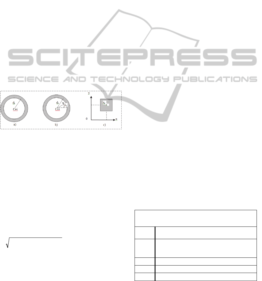
automation sensors. Figure 1 shows the features of
the three types of measurement with the additional
inaccuracy. A ring for goniometric measurement
(Fig.1a), a ring and a cone for goniometric and range
measurement (Fig.1b) and a square band for tactile
tile (Fig.1c).
Figure 1: Measurement type: a) Range, b) Goniometric
and range, c) Tactile tile.
3.1.1 Goniometric Measurement
As said in previous section, the measurement is an
angle λ
i
or λ
j
, the measurement model is given either
by equation (7) or by equation (8) and the inclusion
test is either [f] ([x], [x
i
]) [λ
i
] or [f] ([x],
[x
j
]) [λ
j
] with x
i
the environment sensor
coordinates and x
j
the marker coordinates.
3.1.2 Range Measurement
The measurement is a range d
i
(Fig.1a), the
measurement model is given by g(x)
22
jRjR
yyxx
and the inclusion test is
[g] ([x], [x
i
]) [d
i
].
3.1.3 Goniometric and Range Measurements
The sensor is supposed able to measure both the
angle λi or λj and the range di(Fig.1b) ,the
measurement model is given either by (f
i
(x) or f
j
(x))
and g(x) and the inclusion test is either [f] ([x], [x
i
])
[λ
i
] or [f] ([x], [x
j
]) [λ
j
] and [g] ([x], [x
i
]) [d
i
].
3.1.4 Tactile Tile, Door Crossing Detector
and Complex Shape
The measurement are the coordinates of the center
of the tile(Fig.1c), the measurement model is x
i
= x
R
,
y
i
= y
R
and the inclusion test is [x] [x
i
].
The door crossing detector is a variation on the
tile model. It is considered as a narrow tile in which
the interval associated to each coordinate [x
i
] and
[y
i
] is different.
A complex shape can be considered as a set of
tactile tiles. The measurements are {C
ei
(x
i
, y
i
)} for
i= 1 to n, the measurement model is for i= 1 to n,
x
i
= x
R
, y
i
= y
R
and the inclusion test is for i= 1 to n,
[x] [x
i
].
The literature offers other examples of measure
processing by the set approach for localisation, [18]
with GPS data or (Moore, 1979) with dead
reckoning data. We propose both ways to process
the latter kind of measurement.
3.1.5 Dead Reckoning
The first way is the same as in cases presented
previously. The measurements are x
i
, y
i
,
I
, the
measurement model is x
Rn
= x
Rn-1
+x
n
,
y
Rn
= y
Rn-1
+y
n
,
Rn
=
Rn-1
+
n
at time n and n-1 and
the inclusion test is [x
n
] [x
n-1
] + [x
n
].
3.2 Measurement Synchronisation
There is another way of using dead reckoning data.
When at a given time there are not enough
measurements for an accurate localisation, it is
possible to take account x
i
, y
i
,
I
for
synchronising measurements acquired at different
times.
Algorithm # 3: Inclusion test ([x], [λ
i
], x
i
, t
i
and [dx]).
1
if ( [f] ([x-dx], x
i
, t
i
) [λ
i
]), [x] is
feasible ;
2
else if ([f] ([x-dx], x
i
, t
i
)) [λ
i
] = ), [x]
is
unfeasible ;
3 else [x] is ambiguous ;
4 endif
5 endif
For example let three goniometric measurements
ICINCO2013-10thInternationalConferenceonInformaticsinControl,AutomationandRobotics
134

[λ
n-2
], [λ
n-1
], [λ
n
] acquired at time t
n-2
, t
n-1
, t
n
and [dx
n-
2
], [dx
n-1
] the robot displacement given by odometry
between t
n-2
, t
n-1
andt
n-1
, t
n
respectively. [x] can be
computed at time t
n
taking into account both the
three measurements[λ]and the two relative robot
measurements [dx] by applying the following
inclusion test pour t
i
= t
n-2
or t
n-1
(algorithm #3).
3.3 Processing of Environment Model
Inaccuracies
The forward-backward contractor method uses a set
of variables represented by interval domains with
constraints such as equations (Jaullin et al., 2001).
All equations or equation systems are available even
not invertible ones. Variables may be as well, well-
known input variables as unknown output variables,
because all variables are processed in the same way.
The forward-backward contractor is based on
constraint propagation. This contractor makes it
possible to contract the domains in order to progress
towards the solution and calculate the output
variables (note that input variables may be also
contracted depending on the measurement tolerance
of some input variables); this process is driven by
taking into account any one of the constraints,
proceeding by intersection of intervals. The aim of
propagation technique is to contract as much as
possible the domains of the variables without
loosing any solution.
Consider n variables x
1
,….,x
n
linked by m
constraints C
1
,…., C
m
. For each variable x
i
, it is
assumed that a prior feasible domain [x
i
] = [x
i
-
, x
i
+
]
is known. This domain may be equal to ]-∞,+∞[ if
no information is available on x
i
. Interval algebra
requiring adapted functions, the constraints must be
decomposed into primitive constraints, increasing
the number of equations and of variables. Then each
constraint is calculated according to each variable
using interval intersection. Necessarily, the interval
length will decrease. This operation is repeated
forward and backward until no more significant
contraction can be performed. It can be noted that
contraction is a quick method which in some cases
can slow down or even stop the localisation process
before obtaining the desired accuracy. Contraction
has to be completed by the bisection method.
This method is able to treat a set of
heterogeneous measurement by introducing each
measurement equation as a new constraint. We have
added a forward-backward contractor step to the
bisection algorithm #2 so as to reduce the solution
space and so the computing time.
Moreover the method can reduce the
environment model inaccuracies. In our case, we
assume that home sensors or markers have been
initially approximately located in the home reference
frame. The interval domain associated to their
coordinates can be reduced with further
measurements, either online while detecting outliers,
or offline during a learning phase. This is obtained
by the typical process of the forward-backward
contractor which decreases all interval domains of
each variable, input variable as well as output
variable.
4 SIMULATION RESULTS
The simulation aims at showing: i) the feasibility
and the interest of the localization method whatever
the position of the sensors and the markers, ii) the
ability to integrate a variable number of
measurements, iii) the ability to mix heterogeneous
measurements, iv) the influence of the parameter
on the computing time of localization. The
algorithm is implemented on Matlab software.
4.1 Experimental Protocol
The robot coordinates are specified in the reference
frame. The true measures from the sensors are
computed given the known coordinates of the
sensors and the markers. Then a specified
inaccuracy is added to the measurements in the form
of upper and lower bounds.
4.2 Robot Localisation using
Heterogeneous Measurements
The robot position is represented by two subpavings
which include the set of the solution boxes, the
feasible subpaving in red (or dark grey) and the
ambiguous subpaving in blue/yellow (or light grey).
It is necessary to consider both subpavings to
guarantee a set containing all possible robot location
given the measurements and the noise bounds.
Figure 2 shows the robot position and orientation
(x
R
, y
R
, θ
R
) using three measurements from the robot
onboard sensor which detects three markers labelled
M
i
(Fig.1a). The labels are located at the coordinates
of the markers. Note that in this case the equations
system allows the computing of the robot
orientation.
The simulation parameters are
iiiii
, with Δλ
i
= π/36,
MobileRobotLocalizationbasedonaSetApproachusingHeterogeneousMeasurements
135
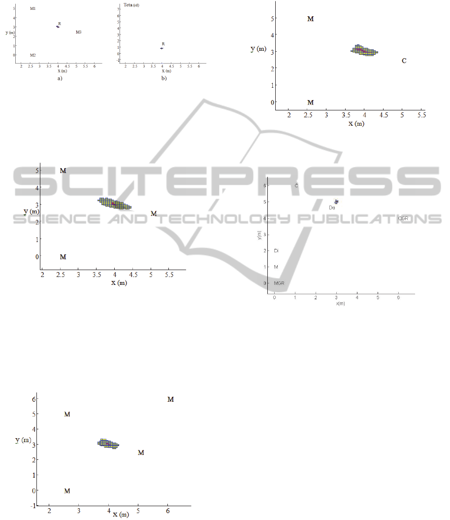
= 0.02 m. The true robot configuration is
(4 m; 3 m, π/4).
Figure 2: 2-DOF robot localization a) Projection on the x-
y plane, b) projection on the x- plane.
For readability only feasible subpaving is
displayed. The results are satisfying in terms of
localization accuracy.
Figure 3: 3-DOF robot localization. Projection in the x-y
plane: With three available measurements.
One of the interests of the approach is the ability
to integrate easily a variable number of
measurements. For example if a fourth measurement
is available, it is added to other measurements for
reducing the localization area (Fig. 4).
Figure 4: 3-DOF robot localization. Projection in the x-y
plane: With four available measurements.
The method can without difficulty include both
goniometric measurements from onboard robot (M)
and from home sensors (C) as illustrated in Figure 5
but also heterogeneous measurements (Fig. 6).
Figure 5: 3-DOF robot localization. Projection in the x-y
plane: One of the measurements is acquired by a home
sensor (C).
Figure 6: 2-DOF robot localization with 6 heterogeneous
measurements.
Label C stands for home goniometric
measurement, M for robot goniometric
measurement, Di for range measurement, CGR for
home range and goniometric measurement, MGR for
robot range and goniometric measurement, Da for
tile measurement. The true robot configuration is
(5; 3) m. The labels are located at the coordinates of
the markers or the sensors.
4.3 Computing Time of Robot
Localisation
In order to verify if the computing time of
localization is compatible with the real time
constraint of robotic application we have realized
two evaluations. The algorithm is implemented on
Matlab software.
The first test evaluates the influence of the
localization accuracy and of the parameter number
on the computing time (Table 1).The simulation
parameters are
iiiii
,
with
ICINCO2013-10thInternationalConferenceonInformaticsinControl,AutomationandRobotics
136

Δλ
i
= π/144, the robot position accuracy
xy
varies
from 0.5 m to 0.001 m, the robot orientation
accuracy
does not change. The room size is 6x6
m
2
.The values of table are the mean time for 100
different positions of the robot. The robot orientation
does not change,
R
= Pi/4. In the first row the 2-dof
robot localization is computed from the
measurements provided by three goniometric
sensors located at (3 ; 0), (0 ; 6), (6 ; 6) m. The
second row gives the mean time needed for the 3-dof
robot localisation. In the latter case the experimental
conditions are the same as for the first row. The only
difference is that one of the three measurements is
necessarily acquired from the robot in order to
calculate the robot orientation.
Table 1: Computing time of the 2-DOF or the 3-DOF
robot localization with respect to the localisation accuracy.
Accuracy (m)
Computing Time (s)
(x
R
, y
R
)
(x
R
, y
R
,
R
)
0.5 0.01 0.24
0.1 0.019 0.44
0.05 0.03 0.22
0.025 0.05 0.22
0.015 0.09 1.44
0.01 0.17 5.29
0.001 1.24
A 2-dof robot localization can be computed
below a second up to 0.01 m accuracy. A 3-dof
robot localization can be computed below a second
up to 0.1 accuracy. The robot orientation is time
consuming.
The second test evaluates the influence of the
number of measurements on the computing time.
The global dimensions of the room are 6m x 6m.
The localization accuracy is = 0.05 m. The robot
coordinates are X = [3 m, 5 m, 1 rd].The position
and the precision of the sensors are randomly
chosen, Δλ
i
[π/72; π/72] . The computing times,
mean and standard deviation, are calculated from of
100 random samplings. As explained before one
measurement is provided by the robot in order to
compute its orientation. We progressively increase
the number of sensors. The added sensors are of the
same type. The Figure 7 gives a representative
example when adding goniometric measurements
acquired by home sensors. Whatever the type of
sensors added the curve has the same shape.
The second evaluation shows that the computing
time depends little on the number of measurements.
It is not necessary to develop a strategy for selecting
among available measurements. We can take all.It
also appears that the standard deviation added to the
sampling of the curves decreases with the number of
measurements. This fact shows that the computing
time is sensor coordinate dependant.
Figure 7: Computing time of the 3-DOF robot localization
with respect to the measurement number.
5 EXPERIMENTAL RESULTS
Real experiments have been performed with a
physical robot in a smart environment composed of
two.
Experiments aim at: i) confirming the simulation
results, ii) showing how outliers could be processed
and, iii) evaluating the influence of the parameter
on the computing time. The algorithm is
implemented on Matlab software.
5.1 Experimental Protocol
The global dimensions of the test bed are 9.4m x
6.4m. The rooms are equipped with presence
sensors, video cameras fixed on the top of the walls,
a pan video camera embarked on the robot and
visual markers. The markers located on the walls are
detected by the robot video camera. The markers
located on the robot are detected by the video
cameras fixed on the walls. The Table 2 gives the
main characteristics of the test bed sensors. The data
of table 2 are used by the algorithm for determining
the inclusion function and the upper and lower
bounds associated to the measurement. For example
the measurement of a presence sensor positioned on
the corner will be
)()( 180135
4.6
0
1
pi
x
y
tg
R
R
j
(9)
and the lower and upper bounds will be
)(),(
180
45
180
45
pipi
ijj
(10)
0,00
0,20
0,40
0,60
0,80
1,00
1,20
1,40
1,60
1,80
2,00
0 5 10 15 20 25
Measurement number
Time (s)
MobileRobotLocalizationbasedonaSetApproachusingHeterogeneousMeasurements
137
(see section 4). It appears that such a presence
sensor covers all the room.
Table 2: Characteristics of the test bed sensors.
Sensors
Presence
sensor
Wall
camera
Robot
camera
Precision (°)
45 5 5
Aperture angle (°) 90
55/2 55/2
Orientation
j
(°)
(see Fig1.b)
135 225 Θ robot
Position (x
j
, y
j
) (m)
(see Fig1.b)
(6.4, 0) (3, 2.20)
(x robot, y
robot)
The robot is positioned at a specified coordinates
(x
R
, y
R
, θ
R
). Measurements are collected by a
gateway which handles the exchanges between the
localisation computer and the smart environment.
5.2 Results
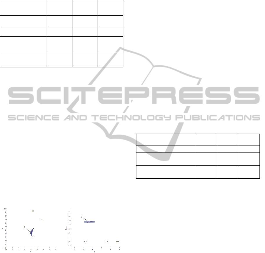
The Figure 8 shows the robot position estimated by
the method from the measurements provided by two
wall cameras (C1, C2). The feasible subpaving is in
red (or dark grey) and the ambiguous subpaving in
blue/yellow (or light grey).The true robot position is
(3, 3.2) 0.2 m is depicted by an ellipse.
A third measurement from the robot video
camera not only improves the position accuracy but
also allows the robot orientation,
R
= 3*pi/2
(Fig.12). C1 and C2 represent the two wall cameras
and M3, the marker detected by the robot video
camera.
Figure 8: 3-DOF robot localization (x,y) in meters and θ in
radians. a) Projection in the x-y plane, b) Projection in the
y- plane.
The results of the real experiments are very close
of those obtained in simulation. Such results are very
useful in poor environment with little sensors
because the robot position and orientation are
modelled as areas. These areas can be more or less
large but it is sure that the robot is inside. Such
information is well-suited to topological space
representation which is more and more used in
robotics in order to simplify databases and be able to
treat various qualities of data. It is a promising result
easy to improve by using a more efficient
programming language.
5.3 Position Map
In order to evaluate a mean computing time for
various relative positions of the robot with the
sensors (C
j
), three home sensors are placed at the
vertices of an equilateral triangle. The robot position
varies from 1 to 6 meters in x and y axis. For each
robot position the set of solution is computed. The
robot orientation is not computed. Real experiments
being more complex to carry out, we have limited
the number of robot positions to ten poses. The robot
poses are equally distributed on the real
environment. Table 3 gives the mean computing
time over ten robot poses for three different
accuracies .
The experiment parameters are: Δλ
i
= π/72.
Table 3: Mean computing time in seconds with respect to
the accuracy for ten robot locations.
Epsilon/accuracy(m) 0.1 0.05 0.01
Mean computing time (s) 0,016 0,027 0,089
Mean measurement
frequency (Hz)
61 37 11
Mean computing time (s)
given by simulation
0.019 0.03 0.17
The results are close to the computing times of
the Table 1 given by simulation. As we said before
the computing time is relatively stable whatever the
robot position in the map related to the sensors. It is
compatible with the real time needs of robotic
application even with a Matlab code.
6 CONCLUSIONS
The robot localization is based on interval analysis
method applied on data both coming from robot and
home sensors. The problem of parameter estimation
is solved by a set inversion applied on error bounded
data. As the parameter vector dimension is two or
three, the computing time is compatible with the real
time constraint of mobile robotics as showed in
sections 4 and 5. The interest of the solution lies on
the ability to integrate a large variety of sensors,
from the roughest to the most complex one.
The method is able to take into account i) a
heterogeneous set of measurements, ii) a flexible
ICINCO2013-10thInternationalConferenceonInformaticsinControl,AutomationandRobotics
138

number of measurements, a statistical knowledge on
the measurements limited to the tolerance; the sensor
model only considers that the measurement is
bounded between the lower and upper limits, iii) the
ability to include measurements both coming from
the robot onboard sensors and from the home
sensors.
The algorithm is able to provide a result of
localization as soon as only one measurement is
available. The results show that the computing time
depends little on the number of measurements. So it
is not necessary to develop a strategy for selecting
among available measurements. We can take all the
available measurements.
The coordinates of the environment markers M
j
=
(x
j
,y
j
) and the coordinates and orientation of the
environment sensors C
j
= (x
j
,y
j
, θ
j
) are supposed
known for paper readability. However the method
we propose can easily take into account inaccuracies
on the marker and sensor coordinates. We also
explain how to handle environment model
inaccuracies.
Works in progress address the case where the
assumption of bounded error is not verified. The
approaches proposed in the literature for processing
outliers have to be improved in order to solve all the
cases.
REFERENCES
Z. Zhang, X. Gao, J. Biswas and J. K. Wu, (2007),
Moving Targets Detection and Localization in Passive
Infrared Sensor Networks, Proceedings of the 10th
International Conference on Information Fusion,
Quebec.
S. Han, H. Lim and J. Lee, (2007), An Efficient
Localization Scheme for a Differential-Driving Mobile
Robot Based on RFID System,” IEEE Transaction on
Industrial Electronics, Vol. 6, 3362-3369.
S. Shenoy and J. Tan, (2005), Simultaneous Localization
and Mobile Robot Navigation in a Hybrid Sensor
Network, Proceedings of IEEE/RSJ International
Conference on Intelligent Robots and Systems,
Alberta.
B.-S. Choi and J.-J.Lee, (2009), Mobile Robot
Localization Scheme Based on RFID and Sonar
Fusion System, Proceedings of IEEE International
Symposium on Industrial Electronics, Seoul, 1035-
1040.
B.-S. Choi and J.-J. Lee, (2010), Sensor Network Based
Localization Algorithm using Fusion Sensor-Agent for
Indoor Service Robot, IEEE Transaction on Consumer
Electronics, Vol. 56, No. 3, 1457-1465.
CorominasMurtra, A., MiratsTur, J.M., Sanfeliu, A.
(2008).Action Evaluation for Mobile Robot Global
Localization in Cooperative Environments, Journal of
Robotics and Autonomous Systems, Special Issue on
Network Robot Systems.
S. Brahim-Belhouari, M. Kieffer, G. Fleury, L. Jaulin and
E. Walter, (2000), Model selection via worst-case
criterion for nonlinear bounded-error estimation,
IEEE Instrumentation and Measurement Vol. 49, No
3
L. Jaulin, M. Kieffer, E. Walter, and D. Meizel, (2002),
Guaranteed Robust Nonlinear Estimation With
Application to Robot Localization, IEEE Trans. SMC,
PartC Applications and Review, Vol. 32 , No 4, 254-
267.
C. Drocourt, (2002). Localization et modélisation de
l'environnement d'un robot mobile par coopération de
deux capteurs omnidirectionnels, thèse.
O. Lévêque, L. Jaullin, D. Meizel and E. Walter,
(1997).Vehicule localization from inaccurate
telemetric data: a set of inversion approach. IFAC
Symposium on robot Control SYROCO 97, Vol. 1,
Nantes, 179-186.
A. Gning,(2006). Fusion multisensorielle ensembliste par
propagation de contraintes sur les intervalles, Thèse.
V. Drevelle and P. Bonnifait, (2010),Robust positioning
using relaxed constraint-propagation. IROS 2010,
Taipei, Vol. 10, 4843-4848.
O. Reynet, L. Jaulin and G. Chabert, (2009), Robust
TDOA Passive Location Using Interval Analysis and
Contractor Programming, Radar, Bordeaux.
L. Jaulin(2009), Robust set-membership state estimation;
application to underwater robotics. Automatica, Vol.
45, No 1, 202–206.
A. Lambert, D. Gruyer, B. Vincke, E. Seignez, (2009),
Consistent Outdoor Vehicle Localization by Bounded-
Error State Estimation, Intelligent Robots and Systems,
IROS
, 1211-1216.
FahedAbdallah, AmadouGning, Philippe Bonnifait,
(2008), Box particle filtering for nonlinear state
estimation using interval analysis, Automatica, Vol.
44, No. 3, 807–815.
R.E. Moore, (1979). Method and applications of internal
analysis, ed. SIAM, Philadelphia.
L. Jaulin and E. Walter,(1993), Set inversion via interval
analysis for nonlinear bounded-error estimation.
Automatica, Vol. 29, No 4,1053–1064.
M. Kieffer, L. Jaulin, E. Walter,(2000), D. Meizel, Robust
autonomous robot localization using interval analysis,
Reliable Computing, Vol. 6, No 3, 337
V. Drevelle P. Bonnifait, (2009),ENC-GNSS 2009
European Navigation Conference - Global Navigation
Satellite Systems, Naples.
L. Jaulin, M. Kieffer, O. Didrit, and E. Walter,
(2001).Applied interval analysis.In Springer-Verlag.
MobileRobotLocalizationbasedonaSetApproachusingHeterogeneousMeasurements
139
