
Cognitive Parameter Adaption in Regular Control Structures
Using Process Knowledge for Parameter Adaption
Martin Schmid
1
, Simon Berger
1
and Gunther Reinhart
2
1
Project Group RMV of Fraunhofer IWU, Beim Glaspalast 5, Augsburg, Germany
2
Institute for Machine Tools and Industrial Management, Technical University Munich, Munich, Germany
Keywords: Modern Control Systems, Adaption, Neural Network, Machine Learning.
Abstract: The colour control system of an offset printing machine is one example, where modern information
processing technologies allow an improved process control and higher resource efficiency. It is not possible
to measure the printing quality during production start. So no regular closed loop control can be used. For
better system behaviour a simulation model is integrated to calculate the printing quality at any time. To get
an optimal process performance, a high simulation quality must be ensured, which includes a compensation
of process simulation inaccuracies as well as variable influences. Therefore a cognitive system is installed,
which measures the most important influences like the used paper and many other process parameters. After
each production the right model parameters will be calculated by identification algorithms. So a data set
with influences and parameters is available. For the next production run the best-fitting parameters for the
simulation model can be calculated by a Neural Network. Additionally wear and deposits, which change the
machine’s performance, can be compensated. The simulation accuracy and the process control quality rises,
which enables a faster run-up. Savings of paper, ink, energy and time allow an economic application of this
control concept.
1 INTRODUCTION
1.1 Linear Control Theories vs.
Methods of Machine Learning
Controllers are often applied in technical devices
and industrial machines. The controller type depends
on the task. In many processes it is sufficient to use
standard PI- or two-level controller. Therefore a
closed control loop is essentiell, what means that the
process output has to be measured permanently and
fed back into the control system.
There exist several concepts to parameterise the
controller to ensure stability and dynamic system
behaviour. Furthermore powerful computer systems,
powerful libraries and high sophisticated software
tools are available to setup a complete controller in
an easy and fast way.
Although conventional controllers can be used
for many applications there are also disadvantages.
To use standard control theories, the developer
needs to know the transfer function of the machine
as well as the process outputs at any time.
Furthermore the system behaviour has to be nearly
time invariant and approximated as linear.
When one of these conditions is not given, more
sophisticated methods have to be taken into account
(Hafner, 2009); (Ramesh, 2002). If there is no
formal system description, machine learning
methods can be used. The most popular type is the
Neural Network (Huang, 1994); (Moon 2008);
(Rangwala, 1989).
A self-learning system has two states in general.
At first it has to be trained with data representing the
desired behaviour, the so called training set. In the
training sequenzce internal parameters or structures
will be changed, till the Neural Network (or all other
types of supervised learning methods) gives similar
values like the training set (Guanyuz, 2012). When
this step is finished, the system can be used to
calculate outputs to familiar or to new inputs. The
quality of the system strongly depends on the
training set. Additionally the optimal net topology
and a successful training period cannot be predicted
at all. If a self-learning component is used in a
control system, the quality of the complete control
system can vary (Rajagopalan, 1996). A
131
Schmid M., Berger S. and Reinhart G..
Cognitive Parameter Adaption in Regular Control Structures - Using Process Knowledge for Parameter Adaption.
DOI: 10.5220/0004427701310138
In Proceedings of the 10th International Conference on Informatics in Control, Automation and Robotics (ICINCO-2013), pages 131-138
ISBN: 978-989-8565-70-9
Copyright
c
2013 SCITEPRESS (Science and Technology Publications, Lda.)
consequence is that the whole system can work
inaccurately or becomes instable. Furthermore it is
difficult to evaluate the quality of the system
(Suzuki, 2011). Moreover there exists only low
knowledge about learning systems in the industry,
because practical applications are implemented only
seldomly in this way.
1.2 Control Structures in Modern
Printing Machines
With powerful web presses paper and foils are
printed in big lots in a short period of time. There
are several control circuits included for printing,
cutting and regulating the speed and position of the
paper web. For the printing quality the so called
optical density is one of the most important control
parameters, which expresses the amount of colour
on the paper and the optical impress of the printed
sheet.
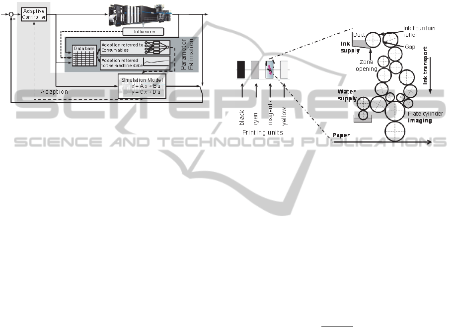
An offset printing machine has four printing
units for each colour black, cyan, magenta and
yellow. Each printing unit is subdivided in up to 40
zones side by side, because the images require
varying amount of ink for each zones. Each zone has
its own ink valve, which can be set individually to
asure the correct amount of ink according to the
printing image. The setting of these valves is called
“zone opening” and can be set through the control
system. The second setting is the speed of the ink
fountain roller, which is equal for all zones. A higher
optical density can be reached by a higher zone
opening or higher roller speed. Both need to be set
correctly to achieve a high printing quality for the
product.
The measurement device for the optical density
needs a specimen field on each sheet. At the
beginning of the printing process the optical density
of this field is too low to be detected by the sensor.
In this time no optical density can be measured and
thus the control circuit is not closed. It is state of the
art to use predefined values at the beginning till the
density is high enough to be detected by the sensor
and close the control circuit. From this point of time
the controllers for the printing quality and the sheet
cutting start working. It has to be considered, that
there are additionally big dead times according to
the machine size, which make the control process
less stable and slower.
The consumables and environmental conditions
like the ambient temperature or humidity also have a
big impact on the printing process.
To prevent an instable behaviour at any time, the
controller is adjusted conservatively. Between start-
up of the machine and reaching the desired optical
density all sheets need to be discarded, because their
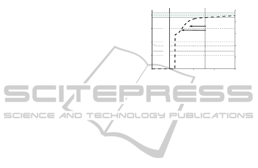
quality level is too low. Figure 1 show the start-up-
period of one zone.
Figure 1: Not acceptable printing quality at the beginning.
The production starts at t = 190 s. At the first 230
seconds no measurements of the optical density are
possible. At t= 500 seconds the optical density is in
the tolerance, so that the product can be sold.
Additionally the zone opening and the ink roller
speed is shown, which stay at a static value at the
beginning.
2 OBJECTIVES
For increasing the resource efficiency and reducing
the production costs, an improved control system is
needed to speed up the starting process for a higher
printing quality in less time. Furthermore, diverse
influences need to be taken into account to heighten
the stability of the control system.
3 APPROACH
3.1 General Concept
To build up a stabil and faster control system it is
essential to get a closed loop, what means, that
output values are available within acceptable time.
In figure 2 all elements of a cognitive model based
control system are shown, which enables these
needs.
A simulation model calculates the output of the
real process in that time, when no measurements can
be taken in the machine. The measured process
output, the optical density, is just needed for
tracking the model to the real printing machine (Rae,
0
20
40
60
80
100
0,0
0,4
0,8
1,2
1,6
0 200 400 600 800
Zone Opening/ Ink Roller Speed
Product Quality (optical density)
Time
Slow rising printing Quality at Production start
s
--
%
Zone Opening
Optical Density
- simulat ed
-measured
Ink Roller Speed
Start of Production at t = 190 s
Tol er an ce
Good Quality
aft er 506 s
ICINCO2013-10thInternationalConferenceonInformaticsinControl,AutomationandRobotics
132
1996). Both, the model and the controller are
conventionally designed as regular linear systems.
Because there are many parameters influencing the
system behaviour, the simulation model needs to be
adjusted to behave like the real machine. For this, a
self-learning adaption mechanism is used to estimate
the real machine parameters on basis of former
productions. The simulation model parameters will
be changed, also like the controller parameters.
Figure 2: Model based control with parameter adaption.
For this, the main influences as well as the
machine settings and the machine outputs are
recorded and compressed to key figures. If a
production is finished, model parameters can be
calculated also, which would have enabled a high
simulation quality in this past production run.
Therefore parameter identification algorithms are
used. These parameters and the influences build up
one dataset for this machine and will be stored in a
data base.
The datasets can be calculated only after a
production. To know the best fitting parameters
before the production it is necessary to determine
them at production start.
For this a statistical adaption to the machine
conditions is implemented. To consider varying
influences machine-learning algorithms are used,
which finds out the optimal simulation model
parameters according to the consumables or the
production conditions.
The model accuracy is higher than an initial
parametrisized model. So the machine reaches its
desired quality level sooner and improves the
resource efficiency.
3.1.1 Real Printing Machine
The printing machine includes four printing units for
each colour. Each unit consists of rollers, which are
mechanically linked via friction to the previous and
next roller, excluding the ink fountain rolle The
number of rollers is necessary to transport and
homogenise the ink film. The ink, stored in the ink
supply, will be transported to the next roller over a
gap. The size of the gap determines a minimum zone
opening to transfer ink onto the next rollers. The
separation between coloured and not coloured areas
occurs on the plate roller, whose surface has
different properties based on the image (Wang,
1984). On the non-coloured areas additional water is
used in the offset printing process. Therefore a water
supply is integrated in the printing unit.
r, which is driven separately. This is shown in figure
3.
Figure 3: Schematic of a printing unit.
3.1.2 Simulation Model
Each touching point between two rollers is called
nip. The mathematical description for the ink flow
between two nips is a first order differential equation
(Kipphan, 2002). For one zone there exist up to 50
nips and a printing unit has up to 50 zones. So the
simulation model for a single printing unit consists
up to 2500 linked differential equations.
To reduce the computational complexity a single
differential equation has been derived for one zone,
describing the behaviour according equation 1.
1
(1)
The input of the system is the zone opening
multiplied with the ink fountain roller speed, the
output is the optical density.
The behaviour of the system is described by the
system gain
, the time constant
and the dead
time
, which regards the delay caused by the ink
transport. The dead time can be calculated via
kinetic and geometric studies. The time constant can
be approximated analytically. The gain consists of
measureable and not measureable components and
describes the static ratio between the machine
settings and the optical density. The gain is affected
by different influencing variables, the consumables
and the machine state and can not be calculated
analytic.
CognitiveParameterAdaptioninRegularControlStructures-UsingProcessKnowledgeforParameterAdaption
133
3.1.3 Influences and Their Clustering
There are four different sources, which may
influence the machine behaviour. The consumables
paper, ink and water can vary. Even consumables,
which should have theoretically the same properties,
can behave differently because of deviations in their
production process or while storage. The machine
ages also, e. g. the rubber of the rollers gets harder
than new ones.
The area coverage is an example of the
influences of the production properties. It is the ratio
between the coloured to the whole area of a sheet in
percent for one zone. If the area coverage is high,
the zone behaves agilely. Otherwise, when the area
coverage is small, the zone behaves inertly. So the
parameters of the printing job have a prevailing
influence. The last types are environmental
parameters. The humidity in the printing room for
example changes the absorbtion rate of the water on
the rollers, which results in a changing optical
impress and density.
3.1.4 Adaptive Controller
When the model will be adapted to the current
machine state, the controller also should be adapted.
A common way is using the model’s parameter
according empirical methods like
Chien/Hrones/Reswick or Ziegler/Nichols. For the
printing process, the method of
Chien/Hrones/Reswick was chosen because of its
robustness and simple implementation (Aström et
al., 2004).
The controller is set only once before the printing
machine starts. If the controller would be tuned
permanently this could cause instability. The
changes of the machine characteristics during run up
are small enough to be neglected.
Like mentioned before each zone has two inputs,
namely the zone valve opening and the speed of the
ink fountain roller. Both values affect the optical
density independently from each other. It is
important to recognise that the zone valve opening
only influences one zone, but the ink fountain roller
speed impacts all zones. Hence a conventional state
space controller can not be applied. To get a linear
control system, both values must be combined to a
virtual machine setting, which can be controlled by a
standard PI-controller. The virtual figure is the
product of the ink fountain roller speed and the zone
opening, corrected by the zone offset. The black line
in figure 4 shows the linear controller output, which
can be achived through a high ink fountain roller
speed and a low zone opening or vise versa.
Figure 4: Variable ratio between ink fountain roller speed
and zone opening.
At the production start (t
start
) a higher ink roller
speed improves the process dynamic. For a stable
process control a higher zone opening has
advantages (t
stationary
). During the ramp up the ratio
between zone opening and ink roller speed changes
for high process dynamics as well as stable
production.
3.2 Higher Simulation Quality
by Analytic Data Mining
In this section it is described how the values of the
minimum zone valve opening can be calculated from
the data of the former lots. The valves of each zone
needs to be opened by an offset, otherwise no colour
is transferred into the printing unit because of a gap
between the ink fountain roller and the following
roller (see figure 5). The offset directly affects the
output of the model. When the offset is high then the
model calculates that only little ink can flow into the
printing unit and the optical density becomes low
and vice versa.
Figure 5: Physical explanation of the offset.
The distance is initial set to 0.08 mm; in reality a
range of 0.03 till 0.10 mm could be measured.
Reasons can be aging or pollution of the mechanical
parts. The gap is implemented to control the ink
roller speed independent from the other rollers
without any friction. Lower zone openings do not
0
20
40
60
80
100
0 20406080100
Ink Roller Speed
Zone Opening
V
ariable Ratio of the Process Input
s
%
Possible process inputs
for one production
%
Offset
t
st a r t
t
st a t i o n a ry
Offset
Distance:
0,03 – 0,1 mm
Pa p er
Ink transport
Ink supply
Zone
Opening
Gap
Ink
Fountain
Roller
Gap
ICINCO2013-10thInternationalConferenceonInformaticsinControl,AutomationandRobotics
134
affect the printing process. This offset makes the
simulation model non-linear and needs to be
considered adequate. Otherwise the model quality
would be too low for the simulation (Eberhard,
2006). This can be done manually, which is very
time consuming. Furthermore the production has to
be stopped for at least three hours to clean and
measure the zone openings. So a method has been
developed to identify the offset by analysing existing
machine data from the prior production runs.
When the optical density has settled then the
zone opening is nearly constant. A higher zone
opening takes more ink on the paper. The amount of
ink can be described via the parameter area
coverage. The higher the area coverage is the more
ink is needed and the higher the zone opening is.
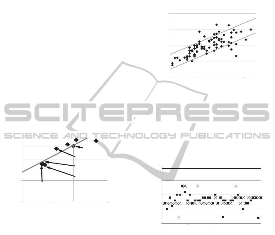
There exists a nearly linear link between the area
coverage and the amount of ink on the paper, shown
in figure 6. For each production ID there is a pair of
area coverage and stationary zone opening.
Figure 6: Zone opening compared with area coverage.
For example the production with the ID 1989 has
an area coverage of 18 % and a zone opening of
52 %.
Figure 7 illustrates this relation for many
productions of a real printing machine. Each dot
represents one production run of a specified zone.
Using numerical methods a best-fit-line can be
generated. When the area coverage is 0% then no
ink is needed. This set point is equal to the offset,
where no colour is transfered into the printing unit
and on the paper.
In practical operation there are also many
operating points, which do not match exactly the
line. To improve the analyses, a 2-step-filter-
method is used. Therefore a first analysis determines
the most probable operating points. A range of
tolerance is definied on this. Only points in this
range are used for the calculation of the best fit line.
According to figure 8 an offset of 18 percent can be
estimated.
Figure 7: Analytical determination of the zone offset.
This method allows determining the actual offset
value, considering dirt and mechanical imperfections
without direct measurements. Figure 8 shows the
comparison between the calculated and the
measured values. The offsets of all 39 zones of the
printing unit cyan are drawn.
Figure 8: Calculated offsets compared with measurements.
The nominal value for the zone offset is 24 %.
The calculated offsets are in a range between 7 and
18 %, the measurements are between 12 and 18 %
and so the accuracy is much better than using the
nominal values. Despites the huge variability of the
real offsets, it is possible to build up an accurate
simulation model without separate measurements.
It has already been shown, that this method
improves the model quality and so increases the
performance of the simulation model.
It needs to be considered that the information
about the offset is just valid as long as no
maintenance is performed or changes in the
mechanics appear. Otherwise the data about the lots
becomes obsolete and new data must get collected to
get right offset values to consider the machine state.
0
20
40
60
0 102030
Stationary Zone Opening
Area Coverage
Raw data for analyti
c
Data M ining
production id: 1823
production id: 1920
production id: ...
production id: 1982
Production id:
1989
%
%
0
20
40
60
80
0 102030
Static zone Opening
Area Coverage
Overview of an 80 % Filter for all
Operation Points in one Zone
%
%
5
10
15
20
25
0 102030
Offset
Zone Number
Comparasion Calculated Values
with Measured Values
Measurement Calculation
%
Nominal value: 24 %
CognitiveParameterAdaptioninRegularControlStructures-UsingProcessKnowledgeforParameterAdaption
135

3.3 Parameter Identification by
Machine Learning Methods
Besides the machine state the consumables and the
process conditions affect the process behaviour. The
simplified simulation model uses a differential
equation to calculate the time behaviour to calculate
the optical density.
3.3.1 Physical Background
The transfer function of the simulation model can be
characterized according equation 1. The model
parameter K
n
can vary corresponding to the physical
variable ink efficiency. This variable is used to
calculate the optical density at specific machine
settings. It is possible to calculate the ink efficiency
on the basis of the measurements afterwards each
production, but not before. An analytic
determination is also not possible, because there are
too many crossactions between process, paper and
ink and moreover the physical and chemical
processes have not yet been identified. This means
finite element analyses are not possible.
Because of this reasons, a multilayer perceptron
(MLP) is used to estimate the ink efficiency on the
basis of the influence parameters (Hintz, 2003). An
MLP is a kind of Neural Network, which consists of
one input and one output layer and several hidden
layers. Each hidden layer is built of neurons (Bayer
et al., 2011); (Beuschel, 2000).
3.3.2 Usage of an MLP to Calculate the Ink
Efficiency
The MLP reproduces the relationship between the
influence parameters and the optimal model
parameters. For this, at first a training period must
be completed successfully (Zell, 1994); (Faridi,
2011). A supervised learning algorithm, that enables
a fast adaption of the network parameters, requires a
training data set, which includes the input
parameters and the corresponding outputs, namely
the parameter ink efficiency. This parameter is
necessary to calculate the model parameter K
n
in
equation 1. The training set is calculated according
former production runs. All measurements will be
analysed and compressed to key figures for the input
variables. The input parameters are the influence
variables like the proberties of the consumables
paper, ink and water, the process conditions like the
temperature and humidity and other physical
characteristics. The corresponding output is the
effective ink efficieny, which can be calculated via
parameter identification algorithms. This is only
possible with completed production runs. The
training period is finished when the net output is
near the desired output. This means, that the net
behaviour is similar to the training sets and thereby
to the machine characteristics.
To use the trained MLP it is necessary to use the
influence parameter of the next production run as net
input. At the start of the production all influence
parameters have to be measured. With these inputs
the MLP can estimate the most probable ink
efficiency for the next production. This enables the
computation of the model parameter K
n
for an
optimal simulation accuracy of the simulation
model. This enables a parameter adaption of the
model and the controller before the start and without
a closed loop control. It is called cognitive parameter
adaption, because only influence variables are used
and combined in a new way.
3.3.3 Topology of the Neural Network
For this application an MLP net was selected
because it is particularly suitable for handling many
inputs. The input and the output data are linearly
normalized due to their physical range of values.
The output neuron has a linear activation function so
that the ink efficiency can be any value between 0.5
and 2.5. All other neurons obtain a sigmoid
activation function. The number of inputs and output
neurons are held constant. The actual structure of the
Neural Network is not predefined.
3.3.4 Topology Optimisation of the Neural
Network
To find the optimal network structure, several
networks with different structures are trained with
the same training data. The networks vary in the
number of hidden layers and in the total number of
neurons. At the end of the training phase the
performance of each network will be evaluated
automatically using a reference data set. The
network with the least error is assumed to have the
best structure and the best ability to generalise, so
this will be used for further calculation of the ink
efficiency.
3.3.5 Workflow
Before the production starts, the simulation model
sends a request to the Neural Network to deliver the
ink efficiency. The network gathers all input values,
calculates the ink efficiency and sends it to the
simulation model. This step takes up to 20 seconds.
ICINCO2013-10thInternationalConferenceonInformaticsinControl,AutomationandRobotics
136
The training and the optimisation of the network
take up to 30 hours. This is not time critical because
the network gets trained only once a month on a
separate computer. If a new production starts while
training, the old network will be used to calculate
the ink efficiency. This means that the training and
the usage is completely separated.
4 RESULTS
4.1 Improvement of the Machine
Behaviour using a Model based
Controller
Until now no dead times are considered in the
controller design. The same can be stated for many
other important influences. So the controller is
designed slowly to avoid unstable behaviour. This
results in a slow system dynamic according to
figure 1. The desired optical density of 1.6 is
reached at t = 500 seconds and so the machine
produces insufficient quality for more than 300
seconds.
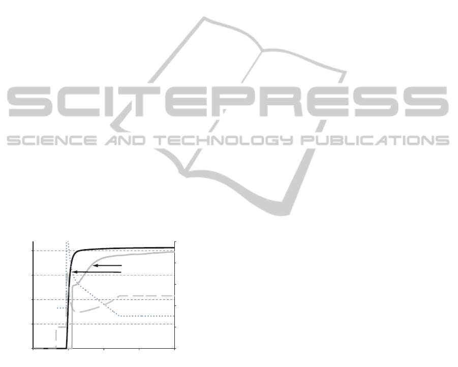
Figure 9 shows the rising of the optical density
using the model based adapted controller. These
values can be compared with figure 1, the controller
and system behaviour is simulated offline.
Figure 9: System dynamic with a model based controller.
At t= 190 seconds the ink roller speed is set to
100 % and the zone opening get up to 70 % for some
seconds and get down after that, so a dynamic ramp
up is possible. Also the variable ratio between zone
opening and roller speed is shown. It can be seen
easily that the machine, which starts at the same
time, just needs 30 seconds to reach good quality.
This means that in this case the efficiency was
increased by the factor of 10 in the simulation. It can
be seen that the density does not overshoot.
4.2 Quality of the Model Adaption
4.2.1 Determining the Zone Offset
The information, which is currently used for the
model, can also be helpful for other purposes. It
could already be proven that the offset in the zone
valve opening has a drift from one side to another
without any visible reasons. This information was
used to demonstrate that an overhaul needs to be
done, which includes cleaning and a mechanical
setup of the zone offsets.
4.2.1 Neural Identification of the Model
Parameter
The Neural Network determines variables, which
cannot be calculated before production start. It needs
to be considered that a Neural Network needs as
many training data sets as possible to cover all
possible variations of the input parameters. The
training sets have to be evenly spread over all
parameters. Furthermore it is also necessary to
substitute old data by new one. This is especially
caused by the aging of the mechanical parts and due
to deposits. Additionally several filters are applied
for the training data, which increases the accuracy of
the data and enables a well-designed network.
5 OUTLOOK AND NEXT STEPS
Most experiments are done on a test printing
machine. Currently it is being integrated into a real
production system. Therefore the model and the
controller have been extended. Furthermore the
Neural Network needs to be optimized so that its
training takes less time. Input parameter with small
effects skipped.
Furthermore the effect of the Neural Network on
the simulation quality has to be determined.
Therefore the real control behaviour with and
without the parameter adaption must be compared.
6 CONCLUSIONS
It is state of the art to apply conventional control
theory for production machines. More powerful
tools like self-learning systems are rejected because
of their non-deterministic behaviour.
To improve the resource efficiency of a printing
machine the capacity of these systems are needed. A
combination of the mathematical deterministic of
0
20
40
60
80
100
0,0
0,4
0,8
1,2
1,6
0 200 400 600 800
Zone Opening/ Ink Roller Speed
Product quality (optical density)
Time
Optimized system Behaviour
with an Adapted Controller
s
--
%
Zone Opening
Optical Densit y
-origin
- controlled
Ink Roller Speed
CognitiveParameterAdaptioninRegularControlStructures-UsingProcessKnowledgeforParameterAdaption
137

analytic controllers with an advanced self-learning
system was developed for a printing machine.
For this machine a transfer function model was
designed which describes the principal behaviour.
To identify the model parameter before the
production start, diverse devices and information
about the consumables and the environmental
conditions are used. All influences, whose
correlation can be described analytically, are also
calculated in that way. Influences with unknown
mode of action are regarded with a Neural Network.
Therefore the most important impacts are measured,
conditioned and fed to the network. So it is possible
to predict the machine’s behaviour under varying
operation conditions with unknown effects. The
simulation model and the controller are turned
according the adapted parameter to guarantee a
stable and dynamic production. This enables higher
product quality and efficiency.
ACKNOWLEDGEMENTS
The authors want to express their gratitude to the
state government of Bavaria for its financial support
of the project “CogSYS – Resource Efficiency by
Cognitive Control Systems”.
REFERENCES
Aström, K. J., Hägglund, T., 2004. Revisiting the Ziegler–
Nichols step response method for PID control.
Bayer, J., Osendorfer, C., Smagt, P., 2011: Learning
Sequence Neighbourhood Metrics. Technical
University Munich.
Beuschel, M., 2000. Neuronale Netze zur Diagnose und
Tilgung von Drehmomentschwingungen am
Verbrennungsmotor, Technical University Munich.
Eberhard, M., 2006. Optimisation of Filtration by
Application of Data Mining Methods, Dissertation,
Technical University Munich.
Faridi, A.; Golian, A., 2011: Use of neural network
models to estimate early egg production in broiler
breeder hens through dietary nutrient intake. In:
Poultry Science.
Govindhasamy, J. J.; McLoone, S. F.; Irwin, George W.;
French, J.; Doyle, R. P., 2005: Neural modelling,
control and optimisation of an industrial grinding
process. In: Control Engineering Practice 13.
Guanyuz, Zhou (2012): Online incremental feature
Learning with denoising autoencoders. International
Conference on Artificial Intelligence and Statistic,
2012.
Hafner, R. 2009: Dateneffiziente selbstlernende neuronale
Regler. University Osnabrück.
Hintz, Christian, 2003: Identifikation nichtlinearer
mechatronischer Systeme mit strukturierten
rekurrenten Netzen. Dissertation. Technical University
München.
Huang, S.H; Hong-Chao Z., 1994: Artificial neural
networks in manufacturing: concepts, applications,
and perspectives. IEEE Trans. Comp., Packag.,
Manufact. Technologies.
Kipphan, H., 2002. Handbuch der Printmedien, Springer
Verlag, Berlin.
Moon, P.; et al. , 2008. Ink-jet printing process modeling
using neural networks. International Electronics
Manufacturing Technology Conference.
Rangwala, S. Dornfeld, D. A., 1989. Learning and
optimization of machining operations using computing
abilities of neural networks, IEEE Transactions on
Systems, Man, and Cybernetics.
Ramesh. R., Mannan M.A., Poo A.N., 2002. Support
vector machines model for Classification of Thermal
Error in Machine Tools, in: The International Journal
of Advanced Manufacturing Technology.
Rajagopalan, Ramesh; Rajagopalan, Purnima, 1996.
Applications of Neural Network in Manufacturing.
International Conference on System Sciences.
Suzuki, K, 2011. Artificial Neural Networks - Industrial
and Control Engineering Applications.
Wang, D., 1984. An investigation of the applicacability of
Walker and Fetsko ink transfer equation, Rochester,
New York.
Rae, T.A; et al, 1996. The application of neural Networks
to induction machine control. Proceedings of IEEE.
Zell, A., 1994. Simulation neuronaler Netze, Oldenburg
Verlag, München.
ICINCO2013-10thInternationalConferenceonInformaticsinControl,AutomationandRobotics
138
