A Generic and Flexible Framework for Selecting Correspondences

in Matching and Alignment Problems

Fabien Duchateau

Universit

e Lyon 1, LIRIS, UMR5205, Lyon, France

Keywords:

Data Integration, Schema Matching, Ontology Alignment, Entity Resolution, Entity Matching, Selection of

Correspondences.

Abstract:

The Web 2.0 and the inexpensive cost of storage have pushed towards an exponential growth in the volume

of collected and produced data. However, the integration of distributed and heterogeneous data sources has

become the bottleneck for many applications, and it therefore still largely relies on manual tasks. One of this

task, named matching or alignment, is the discovery of correspondences, i.e., semantically-equivalent elements

in different data sources. Most approaches which attempt to solve this challenge face the issue of deciding

whether a pair of elements is a correspondence or not, given the similarity value(s) computed for this pair. In

this paper, we propose a generic and ﬂexible framework for selecting the correspondences by relying on the

discriminative similarity values for a pair. Running experiments on a public dataset has demonstrated the im-

provment in terms of quality and the robustness for adding new similarity measures without user intervention

for tuning.

1 INTRODUCTION

Organizations, companies, science labs and Internet

users produce a large amount of data everyday. Fu-

sioning catalogs of products, generating new knowl-

edge from scientiﬁc databases, helping decision-

makers during catastrophic scenarios or creating new

mashups are only a few examples of application that

involve the integration of distributed and heteroge-

neous data sources. Unfortunately, the data integra-

tion task is still largely performed manually, in a

labor-intensive and error-prone process. One of the

basic task when integrating data sources deals with

the discovery of semantically-equivalent elements,

and the link drawn between such elements is a corre-

spondence. Given the nature of the data sources, this

task is referred to as schema matching (Bellahsene

et al., 2011; Bernstein et al., 2011), ontology align-

ment (Euzenat and Shvaiko, 2007; Avesani et al.,

2005) or entity resolution (Fellegi and Sunter, 1969;

Winkler, 2006). An example of schema matching task

which occurs during the creation of a mediation sys-

tem for ﬂight booking is the discovery of correspon-

dences between the Web forms (of the ﬂight compa-

nies) and the mediated schema. A similar problem

involving ontology alignment may be found in query

answering on the Linked Open Data: one needs to un-

derstand the relationships between the concepts and

properties of the ontologies of the knowledge bases to

return complete and minimal query results. In entity

resolution, the merging of two databases about prod-

ucts sold by different companies imply the detection

of identical products.

To tackle these challenges, matching tools apply

a diversity of similarity measures between two ele-

ments to exploit the different information stored in the

data sources. For most of the tools, the values com-

puted by these similarity measures are ﬁnally com-

bined into a global similarity score (Doan et al., 2003;

Aumueller et al., 2005; Christen, 2008; Bozovic and

Vassalos, 2008). This score can be used to rank and

present to the user the top-K candidate correspon-

dences for a given element. A tool can also automat-

ically select the correspondences by comparing this

global score with a threshold. In all cases, this task,

that we further name selection of correspondences,

is therefore crucial in the matching process. Yet, we

advocate that this global score is sufﬁcient neither for

a manual nor for an automatic selection of the corre-

spondences. Indeed, it can reﬂect the strong impact

of similarity measures of the same type if the com-

bination function is not correctly tuned. Besides, the

score aggregates all computed similarity values, al-

though most of them may not be signiﬁcant. Thus,

129

Duchateau F..

A Generic and Flexible Framework for Selecting Correspondences in Matching and Alignment Problems.

DOI: 10.5220/0004430401290137

In Proceedings of the 2nd International Conference on Data Technologies and Applications (DATA-2013), pages 129-137

ISBN: 978-989-8565-67-9

 2013 SCITEPRESS (Science and Technology Publications, Lda.)

applying a threshold on the global score to select cor-

respondences may not be the best solution because

a correct correspondence rarely achieves high values

for all similarity measures. Finally, a similarity mea-

sure returns similarity scores but we usually do not

know its inability for discovering a correspondence.

Many measures are applied in a similar fashion, or on

the same elements. Understanding the ignorance of a

measure is crucial. In addition, the values computed

by the measures may not all be useful. For instance,

most terminological measures return a high similarity

value between mouse and mouse, but these elements

may not be related (one if a reference to the animal

and the other to a computer device). In such case, a

contextual similarity measure may disambiguate the

two words, and the value computed by this contex-

tual measure is discriminative for the pair of elements.

Thus, it is important to measure the ignorance of a

similarity measure. For those reasons, the selection

and the tuning of the similarity measures for select-

ing the correspondences are one of the ten challenges

identiﬁed by Shvaiko and Euzenat (Shvaiko and Eu-

zenat, 2008).

In this paper, we propose a framework which

aims at selecting the correspondences indepen-

dently of the similarity measures. It takes into ac-

count both the ignorance and the differences between

the similarity measures and the discriminative simi-

larity values of a candidate correspondence. In addi-

tion, our approach is ﬂexible when one needs to add

or remove a similarity measure. As a consequence,

no tuning is required from the user to combine the

similarity measures. The main contributions of this

paper can be summarized as follows: (i) a ﬂexible

model for representing similarity measures and com-

puting their dissimilarity and ignorance, (ii) a robust

framework for selecting the correspondences regard-

less of the similarity measures and (iii) the valida-

tion of this approach by using a benchmark with real-

world datasets. The rest of this paper is organized as

follows: Section 2 presents the related work in data

integration, and more speciﬁcally how matching ap-

proaches select the correspondences. Next, we pro-

vide in Section 3 the formal deﬁnitions for our prob-

lem. In Section 4, we describe our framework for se-

lecting correspondences. An experimental validation

is presented in Section 5. Finally, we conclude and

outline future work in Section 6.

2 RELATED WORK

As the matching process covers different but related

domains, these recent books provide the related work

in entity resolution (Talburt, 2011), schema match-

ing (Bellahsene et al., 2011) and ontology align-

ment (Euzenat and Shvaiko, 2007). Schema match-

ing and ontology mainly deal with metadata (e.g., la-

bels, properties, constraints) while entity matching is

at the instance level. Yet, both use similarity mea-

sures to obtain similarity values between metadata or

instances, although the types and nature of the simi-

larity measures may differ. The combination of sim-

ilarity measures and the decision maker for select-

ing a pair as a correspondence is a common issue in

the matching domains.

To combine the results of different similarity mea-

sures, the simplest solution is to use a function (e.g.,

weighted average). For instance, most of the systems

which participate in the Ontology Alignment Eval-

uation Initiative (Euzenat et al., 2011) compute ini-

tial similarity values with terminological, structural or

instance-based measures, and they may reﬁne the re-

sults by applying reasoning. The combination of the

measures may be performed with more complex func-

tion, such as artiﬁcial neural networks (Gracia et al.,

2011). This trend is conﬁrmed in the entity matching

task, where most tools combine the measures with a

numeric or rule-based function (K

opcke and Rahm,

2010). Some approaches dynamically select the mea-

sures to be applied : RiMOM (Li et al., 2009) is a

multiple strategy dynamic ontology matching system

and it selects the best strategy (composed of one or

several similarity measures) to apply according to the

features of the ontologies to be matched. The schema

matcher YAM also dynamically combines similarity

measures according to machine learning techniques

(Duchateau et al., 2009), with the beneﬁt of automat-

ically tuning the thresholds for each measure.

Most matching approaches are based on a thresh-

old to select correspondences. In schema match-

ing, Glue (Doan et al., 2003), COMA++ (Aumueller

et al., 2005), Quickmig (Drumm et al., 2007) or

ASID (Bozovic and Vassalos, 2008) automatically

select their correspondences given a threshold. The

threshold value can be manually tuned, for instance

with a Graphical User Interface as in Agreement

Maker (Cruz et al., 2007). In a similar fashion, the

entity matching approach FEBRL enables users to

choose between a threshold or an automatic selec-

tion based on a nearest neighbor classiﬁer (Chris-

ten, 2008). In (Panse et al., 2013), the authors use

a probabilistic model to minimize the impact of cor-

respondences which have been incorrectly selected.

The ontology alignment system S-Match++ does not

return a global similarity value for a candidate pair

of elements, but the type of relationship between the

elements (e.g., subsomption) (Avesani et al., 2005).

DATA2013-2ndInternationalConferenceonDataManagementTechnologiesandApplications

130

Thus, the decision to select a pair as a correspondence

mainly depends on the result of a SAT solver.

To summarize, our framework aims at tackling is-

sues from the previously described systems. First,

the similarity measures combined by a tool cannot

have the same impact, because some of them are very

similar for computing a score. On the contrary, the

speciﬁcity of other measures should be reﬂected dur-

ing the combination. Thus, our framework includes a

model to classify these measures, and our matching

approach is then independent from these measures,

thus providing more genericity. To avoid the tun-

ing task required by most matching tools, especially

when adding or removing a similarity measure, our

framework should be ﬂexible: the combination of the

similarity measures does not depend on the type of

measure. A last remark deals with the similarity val-

ues: many values are not interesting enough to be ex-

ploited, and candidate correspondences do not obtain

useful scores for all measures. Thus, our framework

is selective because only the most interesting values

should be used to compute a global similarity value

for a candidate correspondence.

3 PRELIMINARIES

In this section, we formally deﬁne the problem and

we present our running example.

3.1 Formalizing the Problem

The matching process deals with data sources, which

can be schemas, ontologies, models and/or a set of

instances. Let us consider a set of data sources D.

A data source d ∈ D is composed of a set of ele-

ments E

, each of them associated with an identi-

ﬁer and attributes. Optionally, these elements may be

linked by relationships. The size of a data source, or

its number of elements, is noted |E

|. The matching

problem consists of discovering correspondences, i.e.,

links between the semantically-equivalent elements

from different data sources. Let us note S the set of

similarity measures used by a tool to discover these

identical elements. To assess a degree of similarity

between two elements e ∈ E

and e

∈ E

, a sim-

ilarity measure sim ∈ S computes a similarity value

sim(e,e

) between these elements as follows:

sim(e,e

) → [0,1]

As explained in (Euzenat and Shvaiko, 2007), we as-

sume that all similarity measures return values which

can be normalized in the range [0,1]. Thus, this def-

inition includes the similarity measures which return

a value in ℜ or those which compute a semantic re-

lationship (e.g., equivalence or hyponymy). Similarly

to most matching approaches, we focus on one to one

matching, i.e., a correspondence only involves two el-

ements from different data sources.

Since a similarity measure mainly exploits a few

properties of the data sources (e.g., an element at-

tribute, the relationship between elements, etc.), the

matching process often applies different similarity

measures, thus producing a similarity matrix. All

similarity values are then combined into a global

similarity score. The combination function may be

complex and require tuning. The set of ﬁnal corre-

spondences between d and d

is noted M (d,d

) and

it contains simple correspondences represented as a

tuple (e, e

). These ﬁnal correspondences are se-

lected among all possible candidate correspondences

(mainly the Cartesian product of E

and E

) ac-

cording to their global similarity score (or conﬁdence

score). This selection is performed manually (e.g.,

by proposing a ranking of the correspondences with

the highest global scores) or automatically (e.g., the

matching process selects the correspondences with a

global score above a given threshold). Note that the

mapping function is not in the scope of this paper.

3.2 Running Example

Based on the previous deﬁnitions, we describe a run-

ning example. For sake of clarity, it has been con-

strained to two data sources d,d

∈ D. Each of

them contains three elements: E

= {a,b, c} and

= {a

}. All possible pairs of elements are

candidate correspondences, for which their similar-

ity has to be veriﬁed. The set of correct correspon-

dences (i.e., provided by an expert) contains two cor-

respondences (a, a

) and (b,b

). To match these two

data sources, we use a set of four similarity mea-

sures S = {sim

,sim

}. Table 1 presents

the similarity matrices of each measure, i.e., the simi-

larity values computed for each pair of elements. For

instance, the pair of elements (a,a

) obtains a simi-

larity value equal to 0.8 with the measure sim

. Next,

we illustrate our framework with this example.

4 A GENERIC FRAMEWORK TO

SELECT CORRESPONDENCES

In this section, we describe our framework to select

and combine the most relevant similarity values for

a given pair of elements regardless of the number of

similarity measures. The basic intuition is that the

AGenericandFlexibleFrameworkforSelectingCorrespondencesinMatchingandAlignmentProblems

131

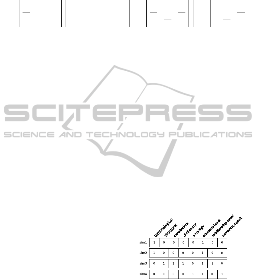
Table 1: Similarity Matrices for Similarity Measures sim

, sim

, and sim

sim

a b c

a’ 0.8 0 0

b’ 0 0.3 0

d’ 0.8 0 0.7

sim

a b c

a’ 0.1 0.1 0.1

b’ 0.2 0.1 0.2

d’ 0.8 0.2 0.6

sim

a b c

a’ 0.6 0.2 0.1

b’ 0.3 0.9 0.4

d’ 0.3 0.2 0.2

sim

a b c

a’ 0 0 0.5

b’ 0 0.5 0

d’ 0 0 0

conﬁdence score of a pair (i.e., the global similar-

ity value) has to reﬂect the presence of discrimina-

tive similarity values for that pair and the diversity

of the types of similarity measures which computed

these similarity values. In other words, a conﬁdence

score should be higher for a candidate correspondence

which obtains discriminative similarity values with

a terminological, a semantic and a constraint-based

measures rather than for a candidate correspondence

which obtains the same values with three terminolog-

ical measures. In the rest of this section, we describe

a model to classify similarity measures and compute

their dissimilarity (Section 4.1). Then, we explain

the meaning of a discriminative similarity value for

a candidate correspondence (Section 4.2). The clas-

siﬁcation model and the discrimination deﬁnition can

ﬁnally be used to compute a conﬁdence score and se-

lect the correspondences (Section 4.3).

4.1 A Model for Comparing Similarity

Measures

Matching approaches combine different types of simi-

larity measures in order to exploit all properties of the

data sources and to increase the chances of discov-

ering correct correspondences (Euzenat and Shvaiko,

2007). However, one needs to correctly tune the

matching tool when possible to avoid that a set of

similar measures (e.g., terminological) has too much

impact in the global similarity score. Indeed, the

types and differences between similarity measures are

rarely taken into account. In addition, their ignorance,

or inability to detect a similarity, is not considered.

For instance, two elements labeled mouse would be

matched with a high score by a terminological mea-

sure, although one of them may refer to as a com-

puter device while the other may stand for an animal.

This is due to the fact that the terminological measure

only uses the string labels to detect a similarity, and

no other information such as external resource, con-

straints, element context, etc. Consequently, the ig-

norance of a similarity measure should reﬂect its lim-

itations in terms of information that it uses to detect

a similarity. Similarity measures have been largely

studied in the literature (Euzenat and Shvaiko, 2007;

Cohen et al., 2003). And a classiﬁcation of these mea-

sures has been proposed (Euzenat et al., 2004) and

later reﬁned (Shvaiko and Euzenat, 2005). In a similar

fashion, we provide a non-exhaustive list of features

of similarity measures:

• the type or category (e.g., terminological, linguis-

tic, structural)

• the type of input (e.g., character strings, records)

• the type of output (e.g., number, semantic rela-

tionship)

• the use of external resources (e.g., a dictionary, an

ontology)

To compare the similarity measures, we propose

to represent them as binary vectors according to their

features. A feature is in our context a property that

the similarity measure fulﬁlls or not. Each similarity

measure sim

∈ S is represented by a binary vector

∈ V . The size of a vector is |v

|, i.e., the number

of features. We can see the set of binary vectors as

a matrix, where f

represents the binary value of the

feature for the i

vector.

In our running example, the four similarity mea-

sures are represented by vectors with 8 features, as

shown in Figure 1. For instance, the third similar-

ity measure is not terminological but it exploits the

structure and the constraints of the data source with a

dictionary as external resource. It is applied against

the elements and the relationships of the data sources.

Figure 1: Binary Vectors for each Similarity Measure.

We ﬁnally obtain a classiﬁcation of the similar-

ity measures. This classiﬁcation not only highlights

the features of the measures but also indicates the ig-

norance of a measure (with respect to the features).

For instance, a terminological measure such as sim

would not detect a similarity between synonyms in

most cases. It is possible to reﬁne the classiﬁcation

by adding more features. The goal is to compute the

DATA2013-2ndInternationalConferenceonDataManagementTechnologiesandApplications

132

differences of each similarity measure with regards to

the other ones. For each binary vector v

∈ V , we

compute its difference score noted ∆

sim

with regards

to the other vectors by applying Formula 1. The main

intuition is that a vector is different from another one

if its features are different. Thus, we analyse each fea-

ture of a vector and we calculate the rate of dissimilar

values in the other vectors for the same feature. Given

a number n of similarity measures and a number g of

features, a difference score ∆

sim

is computed as:

∆

sim

∑

h=1

(

∑

j6=i, j=1

⊕ f

n−1

)

(1)

The function f

⊕ f

is the boolean operation exclu-

sive or, which excludes the possibility of same val-

ues for both features. In other words, it returns 1 if

the boolean features are different, 0 else. If all bi-

nary vectors are identical, the difference score equals

0, but this indicates that the vector representation of

the measures is not detailed enough.

We then normalize this difference score in the

range [0,1] to obtain the dissimilarity of a measure

with regards to others. This normalization is shown

in Formula 2:

dissim

sim

∆

sim

∑

a=1

∆

sim

(2)

The dissimilarity score measures the percentage of

features which are different from other measures. We

note that the following statement holds with the nor-

malization:

∑

sim

∈S

dissim

sim

= 1.

Table 2 provides the difference and dissimilarity

scores for each measure in our example. For in-

stance, the difference score of the similarity measure

sim

equals

+0+

= 0.33. Its dissim-

ilarity score is equal to

0.33

(0.33+0.33+0.67+0.375)

= 0.19.

This means that the similarity measure sim

has 19%

of different features compared to other measures, or

sim

has an ignorance degree equal to 81%.

Table 2: Difference and Dissimilarity Scores of each Mea-

sure.

sim

∆ 0.33 0.33 0.67 0.375

dissim 0.19 0.19 0.40 0.22

4.2 Discriminative Measures

In real-case scenarios, a correct correspondence

would certainly not obtain a high similarity value for

all measures. Therefore, combining the similarity val-

ues of all measures to compute a global score may

not seem suitable. Besides, if a measure returns high

similarity values for most candidate correspondences

(e.g., a measure based on data types), then these high

values may not be useful to disambiguate a conﬂict

between two pairs of elements. Thus, we propose

to discover which similarity measures are discrimi-

native for a candidate correspondence, i.e., the mea-

sures which computed a signiﬁcant value for that cor-

respondence w.r.t. others.

To fulﬁll this goal, we are interested in evaluating

the range inside which a value is considered as dis-

criminative. We use the mean and the standard de-

viation to obtain this range of values. Jain et al. have

demonstrated that these formulas are efﬁcient when

we do not need to estimate their values (Jain et al.,

2005). Besides, the standard deviation is sensitive to

extreme values, i.e., the ones that discriminate. Let

us consider a similarity measure sim

∈ S which has

computed a value for all possible correspondences,

i.e., |E

| × |E

|. We can compute the average µ and

the standard deviation σ of this measure sim

as fol-

lows:

∀e ∈ E

,∀e

∈ E

, µ =

∑

sim

(e,e

)

| × |E

σ =

∑

(sim

(e,e

) − µ)

| × |E

As the standard deviation represents the dispersion of

a value distribution, the range of values close to the

average is given by:

rnd

sim

= [µ − σ, µ + σ]

Note that the lower limit of that range equals to 0 if

µ−σ < 0, and the upper limit is equal to 1 if µ+σ > 1.

The similarity values in the range rnd

sim

do not dis-

criminate a candidate correspondence. Therefore, a

discriminative similarity value for a candidate cor-

respondence (e,e

) should not belong to the range

rnd

sim

. We note γ(e,e

) the set of measures that

discriminate a candidate correspondence, i.e., the

measures that satisfy this condition: ∀sim

,sim

∈

γ(e,e

) ⇐⇒ sim

(e,e

) /∈ rnd

sim

In our example, we can compute the average of the

measure sim

. The nine values have an average and

a standard deviation equal to 0.28 and 0.35 respec-

tively. Consequently, the range of non-discriminative

values is [0,0.63]. For instance, the pair (a,a

) is dis-

criminated by the measure sim

since the value com-

puted for this candidate correspondence (0.8) is not

in that range. Note that all underlined values in the

similarity matrices of Table 1 indicate that the corre-

sponding measure is discriminative for the candidate

correspondence. Thus, γ(a, a

) = {sim

,sim

By selecting a subset of the similarity measures,

we express the fact that the discriminative similarity

AGenericandFlexibleFrameworkforSelectingCorrespondencesinMatchingandAlignmentProblems

133

values have more impact than others during the cor-

respondences selection. However, a candidate corre-

spondence may not have any discriminative values in

the ﬁrst round, and thus it is not considered for com-

puting its conﬁdence score. To identify the discrimi-

native measures for such candidate correspondences,

we iterate the process by noting γ

(e,e

) the k

itera-

tion of this process. At the end of each step, the previ-

ous similarity values are discarded, and we compute a

new average and standard deviation, thus generating

a set of new discriminative measures (or an empty

set). This set is then merged into Γ

(e,e

) as shown

with this formula:

(e,e

) =

[

k=1

(e,e

)

The question is how to determine a value for the num-

ber of iterations t. We can use the same techniques

than the matching tools such as a threshold value (i.e.,

there is no more iteration if the average of similarity

values reaches a threshold value) or the ﬁrst k itera-

tions. We can also iterate until all elements of a data

source have been discriminated by at least one mea-

sure, and/or when an iteration has no more discrimi-

native values to propose.

Let us compute the set of discriminative measures

for the second iteration in our running example. We

ﬁrst discard the discriminative similarity values from

the matrices that were previously identiﬁed (i.e., the

underlined values). What happens for the similarity

measure sim

? The new average and standard de-

viation computed for the remaining 6 values equals

0.04 and 0.24 respectively. The similarity value 0.3

for (b,b

) is a discriminative value at this iteration.

Consequently, sim

is added in the set of discrim-

inative measures for the candidate correspondence

(b,b

) and Γ

(b,b

) = {sim

,sim

4.3 Computing a Conﬁdence Score

The next step deals with the computation of a con-

ﬁdence score for a given candidate correspondence.

This score is based on the discriminative similarity

measures and their associated value. Indeed, the in-

tuition is that we should be conﬁdent in a correspon-

dence which obtains high similarity values computed

by distinct and low-ignorance measures. Given a pair

m = (e,e

) and its discriminative similarity values

< sim

(e,e

),.. ., sim

(e,e

) > with sim

,.. ., sim

∈

(e,e

), the conﬁdence score con f

(e,e

) for the t

iteration is calculated as follows:

con f

(e,e

)

∑

i=1

dissim

sim

∑

i=1

sim

(e,e

)

In this formula, we average the discriminative simi-

larity values and we multiply the result by the sum of

all dissimilarities of the measures. As both are in the

range [0,1], the conﬁdence score also has values in the

range [0, 1]. Note that our formula is also a weighted

average like in other approaches, however it does not

require any tuning due to the independence and the

model for the similarity measures.

Back to our example, we can compute the conﬁ-

dence scores of all candidate correspondences which

have discriminative values at the ﬁrst iteration. That

is, the pairs (a, a’), (a, d’), (b, b’), (c, a’), and (c,

d’). Let us detail the probability for the ﬁrst pair to be

correct:

con f (a,a

) = (0.19 + 0.40) ×

0.8 + 0.6

= 0.41

The conﬁdence score for the other candidate corre-

spondences are: conf(a, d’) = 0.30, conf(b, b’) =

0.43, conf(c, a’) = 0.19, and conf(c, d’) = 0.25. We

notice that although the similarity values for the pairs

(a, a’) and (a, d’) are close, we have more conﬁ-

dence in the former pair since it obtains discrimina-

tive similarity values with more dissimilar similarity

measures. The candidate correspondence (c, a’) is

penalized by sim

since this measure mainly computes

high similarity values, except for this candidate pair.

4.4 Discussion

We ﬁnally discuss several points of our approach:

• When the conﬁdence scores of two correspon-

dences involving the same element are very

close, they can be part of a complex correspon-

dence. This needs to be checked by using reﬁned

techniques to discover these complex correspon-

dences (Bilke and Naumann, 2005; Dhamankar

et al., 2004; Saleem and Bellahsene, 2009).

• The boolean features are produced objectively.

Designers or users of a similarity measure knows

whether the measure satisﬁes a feature or not. A

challenging perspective is the automatic deﬁnition

of the binary vector. In the OAEI track bench-

mark

, the objective is to detect the ability of a

matching tool by duplicating a dataset with a mi-

nor change (e.g., changing the language, or delet-

ing the annotations) (Euzenat et al., 2011). By

applying a similarity measure to this OAEI track,

one is able to check if the measure is resistant to

the change, and thus can compute the binary vec-

tor of that similarity measure.

Ontology Alignement Evaluation Initiative (January

2013), http://oaei.ontologymatching.org/

DATA2013-2ndInternationalConferenceonDataManagementTechnologiesandApplications

134

• In the current version, we use binary vectors,

which means that a measure owns the feature or

not. We could relax this binary constraint by al-

lowing real values. In that case, the vector shows

the probability that the measure satisﬁes the fea-

ture, or the degree of ignorance for the feature.

However, such a modiﬁcation has an impact on

the difference score formula.

• If we do not discriminate the similarity measures

for a given candidate correspondence, the conﬁ-

dence score would be equal to the average of all

similarity values computed for that candidate cor-

respondence.

• It is possible that all similarity measures have the

same similarity score, despite their different fea-

tures. For instance, the four similarity measures

of the running example could have obtained each

a score equal to 0.25. In such case, the dissimi-

larity scores still have a signiﬁcant impact, since

they are used only for the discriminative values

that have been calculated.

• Our approach can be plugged into most match-

ing approaches, especially those that computes a

global similarity score. Our conﬁdence score may

be used to select correspondences either manu-

ally (the user can select within the list of top-k

correspondences based on their conﬁdence score)

or automatically (all conﬁdence scores above a

threshold are returned). Besides, our conﬁdence

score reﬂects the types and ignorance of the simi-

larity measures which have computed the discrim-

inative similarity values.

• Finally, our approach does not require any tuning

for combining the similarity measures, because

we select the values computed by similarity mea-

sures if they are sufﬁciently discriminative.

5 EVALUATION

In this section, we validate our approach in an En-

tity Matching context. We ﬁrst describe the evalua-

tion protocol (benchmark and another tool), then we

compare our approach with another entity matching

tool in terms of matching quality, and we ﬁnally show

the robustness of our approach when adding new sim-

ilarity measures.

5.1 Evaluation Protocol

To demonstrate the beneﬁts of our framework, we

have implemented it and tested against a benchmark

for entity resolution (Kopcke et al., 2010). This

benchmark

contains four datasets and has been eval-

uated by their authors with a matching tool (whose

name is unknown due to licensing). We refer to this

matching tool as BenchTool in the rest of the paper.

The four datasets mainly cover two domains: Web

products (Abt-Buy and Amazon-GoogleProducts) and

publications (DBLP-Scholar and DBLP-ACM). The

size of the data sources contained in these datasets

vary from 1081 (Abt) entities to 64283 (Scholar),

with an average around 2000 entities. The set of per-

fect correspondences is provided for each dataset and

their size varies from 1097 (Abt-Buy) to 5347 (DBLP-

Scholar) (Kopcke et al., 2010). The matching quality

is computed with the three well-known metrics (Eu-

zenat and Shvaiko, 2007; Bellahsene et al., 2011).

Precision calculates the proportion of relevant corre-

spondences among the discovered ones. Recall com-

putes the proportion of correct discovered correspon-

dences among all correct ones. Finally, the F-measure

evaluates the harmonic mean between precision and

recall. Since both tools obtain a score for these met-

rics which is close to the F-measure (e.g., precision

equal to 97%, recall to 95% and F-measure at 96%),

we only present the plots for the F-measure.

The conﬁguration of our framework is as follows.

We have 5 similarity measures : three of them are ter-

minological (Jaro Winkler, Monge Elkan, Smith Wa-

terman from the Second String API

), another one is

based on the frequency of the words in ﬁelds such as

description or title (Duchateau et al., 2009), and the

last one is the Resnik measure applied to the Word-

net dictionary (Resnik, 1999). All these measures

have been classiﬁed with the 8 features described in

Section 4.1. The number of iterations is limited to 2

and the conditions for selecting a correspondence is a

combination of threshold and top-1: for each element

from the source, its correspondence is the candidate

correspondence with the best conﬁdence score only

if this score is above a threshold. This threshold is

computed by averaging all similarity values. For the

BenchTool, we assume that the best tuning was per-

formed by the authors when they ran it against the

Entity Matching Benchmark (Kopcke et al., 2010).

5.2 A Quality Comparison with

BenchTool

Our ﬁrst experiment aims at showing the matching

quality obtained by our approach with regards to the

BenchTool approach. Figure 2 depicts the results of

Entity Matching benchmark (January 2013), http://

dbs.uni-leipzig.de/en/research/projects/object matching/

API at http://secondstring.sourceforge.net/

AGenericandFlexibleFrameworkforSelectingCorrespondencesinMatchingandAlignmentProblems

135

BenchTool

OurApproach

100

DBLP−ACM DBLP−Scholar Abt−Buy Amazon−GP

F−measure Value

Figure 2: Results of BenchTool and our approach in terms

of F-measure for the 4 datasets.

the two systems for the four datasets. For the publica-

tions datasets, which are easier to match, both tools

obtain an acceptable matching quality and our ap-

proach achieves a F-measure score above 95%. The

products datasets are more difﬁcult to match for two

reasons: ﬁrst, a description ﬁeld is confusing because

it contains either full sentences or sets of keywords.

Secondly, two products may slightly differ (e.g, two

hard drives of different size from the same manufac-

turer). For these datasets, BenchTool obtains a F-

measure around 60 − 65%. Our approach performs

better with a F-measure between 70% to 78%. Al-

though our tool was not speciﬁcally designed for the

entity matching task, we note that it achieves a bet-

ter F-measure for all datasets. This means that our

generic framework for selecting correspondences in-

dependently from the similarity measures is effective.

5.3 Demonstrating Robustness

and Flexibility

In a second experiment, we demonstrate the robust-

ness and the ﬂexibility of our approach regardless of

the similarity measures. A majority of matching ap-

proaches requires some tuning for combining similar-

ity measures (e.g., setting weights). Thus, when a new

similarity measure is added, it is necessary to recon-

ﬁgure the tool. Since our framework considers each

similarity measure individually, there is no need for

tuning

and we demonstrate that the matching quality

does not decrease when adding more measures. We

have compared the variation of the F-measure value

when increasing the number of similarity measures.

To perform this experiment, ﬁve measures from the

Second String API have been added (e.g., Afﬁne Gap,

The similarity measure has to be described according

to the boolean features, which is still simpler than tuning a

combination function. And such description can be shared

and reused in an ontology for instance.

100

0 1 2 3 4 5 6 7 8 9 10

F-measure

Number of similarity measures

DBLP-ACM

DBLP-Scholar

Abt-Buy

Amazon-GP

Figure 3: Results of our approach for the 4 datasets when

varying the number of similarity measures.

Jaccard), and the measures have been randomly se-

lected. We have run this experiment 10 times for each

dataset to limit the impact of the randomness. Fig-

ure 3 illustrates the average F-measure (of all runs)

for the four datasets with various number of similar-

ity measures. When adding more measures and with-

out any tuning, the trend of the plots is an increase or

stabilization of the F-measure value. For the DBLP-

Scholar dataset, the F-measure value is equal to 70%

with one measure, and then it increases to reach 98%

with 10 measures. For the products datasets, the 5

terminological measures which have been added are

not sufﬁcient to improve strongly the results. Other

types of similarity measures are necessary to increase

the matching quality of these datasets. To conclude,

our framework is robust and ﬂexible to the number of

similarity measures that can be added without tuning.

6 CONCLUSIONS

In this paper, we have proposed a novel framework

for selecting correspondences in a matching or ontol-

ogy problem. Contrary to other approaches, our ap-

proach does not require any tuning to combine those

measures. The experiments against an entity reso-

lution benchmark have demonstrated both the major

improvement of our approach in terms of quality and

its robustness regardless of the number of similarity

measures involved in the matching. As for the per-

spectives, we plan to perform more experiments, both

with other data integration tasks (schema matching,

ontology alignment) and with various conﬁgurations

of the parameters (number of iterations, number of

features). Although the deﬁnition of features for the

similarity measures can be designed in an ontology

and shared with others users, it would be interesting

DATA2013-2ndInternationalConferenceonDataManagementTechnologiesandApplications

136

to automatically compute the dissimilarity scores, for

instance by analyzing the distribution values of the

measures. Converting the binary vectors into real-

valued vectors would reﬁne the degree of ignorance

of the measures. Such vectors may be computed with

speciﬁc datasets, in which a minor change reﬂects a

feature.

REFERENCES

Aumueller, D., Do, H. H., Massmann, S., and Rahm,

E. (2005). Schema and ontology matching with

COMA++. In ACM SIGMOD, pages 906–908.

Avesani, P., Giunchiglia, F., and Yatskevich, M. (2005). A

large scale taxonomy mapping evaluation. In Interna-

tional Semantic Web Conference, pages 67–81.

Bellahsene, Z., Bonifati, A., and Rahm, E. (2011). Schema

Matching and Mapping. Springer-Verlag, Heidelberg.

Bernstein, P. A., Madhavan, J., and Rahm, E. (2011).

Generic schema matching, ten years later. PVLDB,

4(11):695–701.

Bilke, A. and Naumann, F. (2005). Schema matching using

duplicates. ICDE, 0:69–80.

Bozovic, N. and Vassalos, V. (2008). Two-phase schema

matching in real world relational databases. In ICDE

Workshops, pages 290–296.

Christen, P. (2008). Febrl -: an open source data clean-

ing, deduplication and record linkage system with a

graphical user interface. In SIGKDD International

Conference on Knowledge Discovery and Datamin-

ing, KDD’08, pages 1065–1068. ACM.

Cohen, W., Ravikumar, P., and Fienberg, S. (2003). A com-

parison of string distance metrics for name-matching

tasks. In In Proceedings of the IJCAI-2003.

Cruz, I. F., Sunna, W., Makar, N., and Bathala, S. (2007).

A visual tool for ontology alignment to enable geospa-

tial interoperability. J. Vis. Lang. Comput., 18(3):230–

254.

Dhamankar, R., Lee, Y., Doan, A., Halevy, A., and Domin-

gos, P. (2004). iMAP: Discovering Complex Semantic

Matches between Database Schemas. In ACM SIG-

MOD, pages 383–394.

Doan, A., Madhavan, J., Dhamankar, R., Domingos, P., and

Halevy, A. Y. (2003). Learning to match ontologies

on the semantic web. VLDB J., 12(4):303–319.

Drumm, C., Schmitt, M., Do, H. H., and Rahm, E. (2007).

Quickmig: automatic schema matching for data mi-

gration projects. In CIKM, pages 107–116. ACM.

Duchateau, F., Coletta, R., Bellahsene, Z., and Miller, R. J.

(2009). (Not) Yet Another Matcher. In CIKM, pages

1537–1540.

Euzenat, J. et al. (2004). State of the art on ontology match-

ing. Technical Report KWEB/2004/D2.2.3/v1.2,

Knowledge Web.

Euzenat, J., Ferrara, A., van Hage, W. R., Hollink, L., Meil-

icke, C., Nikolov, A., Ritze, D., Scharffe, F., Shvaiko,

P., Stuckenschmidt, H., Sv

ab-Zamazal, O., and dos

Santos, C. T. (2011). Results of the ontology align-

ment evaluation initiative 2011. In OM.

Euzenat, J. and Shvaiko, P. (2007). Ontology matching.

Springer-Verlag, Heidelberg (DE).

Fellegi, I. P. and Sunter, A. B. (1969). A theory for record

linkage. Journal of the American Statistical Associa-

tion, 64:1183–1210.

Gracia, J., Bernad, J., and Mena, E. (2011). Ontology

matching with cider: evaluation report for oaei 2011.

In OM.

Jain, A., Nandakumar, K., and Ross, A. (2005). Score nor-

malization in multimodal biometric systems. Pattern

Recognition, 38(12):2270–2285.

opcke, H. and Rahm, E. (2010). Frameworks for entity

matching: A comparison. Data Knowl. Eng., 69:197–

210.

Kopcke, H., Thor, A., and Rahm, E. (2010). Learning-based

approaches for matching web data entities. IEEE In-

ternet Computing, 14(4):23–31.

Li, J., Tang, J., Li, Y., and Luo, Q. (2009). Rimom: A dy-

namic multistrategy ontology alignment framework.

IEEE Trans. on Knowl. and Data Eng., 21(8):1218–

1232.

Panse, F., Ritter, N., and van Keulen, M. (2013). Indeter-

ministic handling of uncertain decisions in deduplica-

tion. Journal of Data and Information Quality.

Resnik, P. (1999). Semantic similarity in a taxonomy:

An information-based measure and its application to

problems of ambiguity in natural language. Journal

of Artiﬁcial Intelligence Research, 11:95–130.

Saleem, K. and Bellahsene, Z. (2009). Complex schema

match discovery and validation through collaboration.

In OTM Conferences (1), pages 406–413.

Shvaiko, P. and Euzenat, J. (2005). A survey of schema-

based matching approaches. Journal of Data Seman-

tics IV, pages 146–171.

Shvaiko, P. and Euzenat, J. (2008). Ten challenges for ontol-

ogy matching. In OTM Conferences (2), pages 1164–

1182.

Talburt, J. R. (2011). Entity Resolution and Information

Quality. Elsevier.

Winkler, W. E. (2006). Overview of record linkage and cur-

rent research directions. Technical report, Bureau of

the Census.

AGenericandFlexibleFrameworkforSelectingCorrespondencesinMatchingandAlignmentProblems

137