
Advanced Analytics with the SAP HANA Database
Philipp Große
1
, Wolfgang Lehner
2
and Norman May
1
1
SAP AG, Dietmar-Hopp-Allee 16, Walldorf, Germany
2
TU Dresden, N
¨
othnitzer Str. 46, Dresden, Germany
Keywords:
MapReduce, Advanced Analytics, Machine Learning, Data Mining, In-memory Database.
Abstract:
Complex database applications require complex custom logic to be executed in the database kernel. Traditional
relational databases lack an easy to-use programming model to implement and tune such user defined code,
which motivates developers to use MapReduce instead of traditional database systems. In this paper we
discuss four processing patterns in the context of the distributed SAP HANA database that even go beyond
the classic MapReduce paradigm. We illustrate them using some typical Machine Learning algorithms and
present experimental results that demonstrate how the data flows scale out with the number of parallel tasks.
1 INTRODUCTION
There is a wide range of sophisticated business anal-
ysis and application logic—e.g., algorithms from the
field of Data Mining and Machine Learning—, which
is not easily expressed with the means of relational
database systems and standard SQL. This is particu-
lar true for algorithms such as basked analysis or data
mining algorithms, which are typically not part of the
database core engine.
To realize such algorithms MapReduce as a pro-
gramming paradigm (Dean and Ghemawat, 2004) and
frameworks like Hadoop scaling the Map and Reduce
tasks out to hundred and thousand of machine have
become very popular (Apache Mahout, 2013).
However, the data of most companies are still
primarily located in (distributed) relational databases
systems. Those distributed database systems—like
the SAP HANA database (Sikka et al., 2012)—have
their own means to efficiently support the scale out
of queries. Instead of operating on a key-value store
organized through a distributed file system, the SAP
HANA database operates on in-memory tables orga-
nized through a distributed relational database sys-
tem. However, both have in common that execution
plans can be distributed over a number of different
machines and work will be orchestrated by the over-
all system.
Nevertheless databases have failed in the past to
provide an easy to use programming paradigm for the
parallel execution of first-order functions.
In contrast to this, MapReduce as a programming
paradigm provides a simple to use yet very powerful
abstraction through two second-order functions: Map
and Reduce. As such, they allow to define single se-
quentially processed tasks while at the same time hid-
ing many of the framework details of how those tasks
are parallelized and scaled out.
However, classic MapReduce frameworks like
Hadoop are missing support for data schemas and
native database operations such as joins. Further-
more the lack of knowledge on the framework side
and the required context switches between the appli-
cation layer and the parallel processing framework
makes optimizations, as they are commonly applied
in databases, very difficult if not impossible.
From performance perspective it would be desir-
able to have a tightly integration of the custom logic
into the core of the database. But this would require
hard coding the algorithm into the core and thereby
limiting the extensibility and adaptability of the algo-
rithm integrated.
In this paper we will outline that the SAP HANA
database with its distributed execution goes be-
yond the expressiveness of the classic MapReduce
paradigm, adding the advantage of processing first-
order functions inside a relational database system.
Instead of integrating Hadoop MapReduce into the
database, we rely on a native execution of custom
code inside the database.
The contributions in this paper are summarized as
follows:
• We characterize four different processing pattern
found in Machine Learning and Data Mining ap-
61
Große P., Lehner W. and May N..
Advanced Analytics with the SAP HANA Database.
DOI: 10.5220/0004430800610071
In Proceedings of the 2nd International Conference on Data Technologies and Applications (DATA-2013), pages 61-71
ISBN: 978-989-8565-67-9
Copyright
c
2013 SCITEPRESS (Science and Technology Publications, Lda.)

plications and discuss their mapping to MapRe-
duce.
• We describe a flexible parallel processing frame-
work as part of the SAP HANA database and a
number of basic programming skeletons to ex-
ploit the framework for the different processing
patterns discussed.
• We implement each of the four processing pat-
terns using the basic programming skeletons and
evaluated them using real-world data.
The remainder of this paper is structured as fol-
lows. In section 2 we derive four different processing
patterns to map out the requirements of supporting so-
phisticated business analysis and application logic.
This is followed by section 3, where we discuss
how the presented processing pattern can be applied
in the context of the SAP HANA database. In sec-
tion 4 we present the evaluation of our approach and
discuss in section 5 related work.
2 MACHINE LEARNING
AND MapReduce
To support application developers to implement com-
plex algorithms, we present four basic processing pat-
tern commonly found in standard machine learning
algorithms. Many standard machine learning (ML)
algorithms follow one of a few canonical data pro-
cessing patterns (Gillick et al., 2006), (Chu et al.,
2006), which we will discuss in the context of the
MapReduce paradigm.
• Single-pass: where data has to be read only once.
• Cross Apply: where multiple data sources have to
be considered and jointly processed.
• Repeated-pass: where data has to be read and ad-
justed iteratively.
• Cross Apply Repeated-pass: where the iterative
adjustment has to be processed on multiple data
sources.
To the best of our knowledge the two processing
patterns ’Cross Apply’ and ’Cross Apply Repeated-
pass’ have never been discussed before as full-fledged
patterns in the context of Machine Learning and
MapReduce and are therefore new.
2.1 Single-pass
Many ML applications make only one pass through
a data set, extracting relevant statistics for later use
during inference. These applications often fit per-
fectly into the MapReduce abstraction, encapsulating
the extraction of local contributions to the Map task,
then combining those contributions to compute rele-
vant statistics about the dataset as a whole in the Re-
duce task.
For instance, estimating parameters for a naive
Bayes classifier requires counting occurrences in the
training data and therefore needs only a single pass
through the data set. In this case feature extraction
is often computation-intensive, the Reduce task, how-
ever, remains a summation of each (feature, label) en-
vironment pair.
01. for all classes c
i
∈ c
1
,...,c
m
02. for all documents x
k
∈ x
1
,...,x
n
of class c
i
03. for all feature l
j
∈ l
1
,...,l
v
of document x
k
04. sum
k
(l
j
) = count(l
j
);
05. od;
06. od;
MAP
07. for all feature l
j
∈ l
1
,...,l
v
in all x of class c
i
08. tsum
j
=
∑
n
k=1
sum
k
(l
j
);
09. µ
j
= tsum
j
/count(x|c
i
);
10. for k ∈ 1,...,n
11. di f f
k
= (sum
k
(l
j
) − µ
j
)
2
12. od;
13. σ
j
=
p
1/(n − 1) ∗
∑
n
k=1
di f f
k
14. G
j
= N (µ
j
,σ
j
)
15. od;
16. M
i
=
S
v
j=1
G
j
REDUCE
17. od;
Script 1: Pseudo code to calculate Gaussian distributions
for a set of features and different classes.
To illustrate this: let us assume we want to train a
very rudimental language detector, using some sam-
ple text documents each labeled with its respective
language. To keep things very simple we train a
naive Bayes classifier based on the letter distribution
each language has and assume an equal prior prob-
ability for each language and documents of normal-
ized length. The Bayes classifier relies on the Bayes
theorem, whereby P(A|B) = P(A) ∗ P(B|A)/P(B). In
order to be able to predict the probability P(c
i
|x
k
) of
a language (i.e., class c
i
) given a document (i.e., ob-
servation x
k
), we need to train a model M
i
for each
language, which helps us to calculate the probability
P(x
k
|c
i
) for an observation x
k
given the class c
i
. A
very simple way to represent such a model is by us-
ing Gaussian distributions. Script 1 shows the Pseudo
code for calculating a set of Gaussian distributions to
represent such a model. The training task based on
the letter distribution of documents is very similar to
the well known word count example usually found for
MapReduce. We can distribute our sample documents
equally over a number of Map jobs. Each Map job
DATA2013-2ndInternationalConferenceonDataManagementTechnologiesandApplications
62
will count the number of occurrences for each letter
l
j
returning the letter distribution of the document x
k
.
The key value we use to pass our Map results to the
Reduce job is the language label c
i
of each text docu-
ment, so ideally we will have as many Reduce jobs as
we have different languages, respectively classes, in
our training set. The task of the Reduce job is to ag-
gregate the statistics gained for each document x
k
by
summarizing the results in a statistic model M
i
. As
we use Gaussian distributions to model M
i
for lan-
guage i, the language will be described by the means
µ
j
and standard deviations σ
j
for each letter l
j
in the
alphabet. Based on those Gaussian distribution mod-
els, we can calculate the probability P(x
k
|c
i
) for an
unlabeled document x
k
, which is—as we will see in
section 2.2—the basis for our naive Bayes classifier.
2.2 Cross Apply
A second class of ML applications repeatedly apply
the same logic on a set of models or reference data,
while broadcasting the other. There is only a very
small yet very distinctive difference compared to the
first class of Single-pass algorithms: The aspect of
broadcasting. The repeated apply without the need to
loop is perfectly suited for the MapReduce paradigm,
but the broadcasting aspect introduces a new chal-
lenge. It effectively means that a set of data, respec-
tively models, has to be copied to a number of paral-
lel working threads independent of the data distribu-
tion of the main data set. This requirement of mul-
tiple independent data sets is not properly supported
in most MapReduce frameworks and therefore usu-
ally involves an additional preprocessing step to bun-
dle the data sets under common keys and introduce
custom logic to distinguish between them.
The Cross Apply pattern can be found in a number
of ML concepts such as model choice or meta classi-
fication, where multiple ML models are applied to the
same data. The data is duplicated and each Map task
processes a different ML model, or even the same ML
model with different configuration parameters. The
Reduce task is used to pick the best model, does a
majority vote of the Map results or aggregates the re-
sults for a final classification result. In any of those
cases, sharing common data over a number of Map
jobs is essential. Besides the broadcasting another
difference to our previous Single-pass pattern is that
in those scenarios there is no need for multiple paral-
lel reduce operations, but rather one central decision
maker collecting the results of all the Map jobs. Ap-
plying this pattern not only for a single classification
or model choice task but a number of them, we again
end up with the same data distribution using multiple
Reduce jobs. The same pattern can also be found in
query-based algorithms like nearest neighbor classi-
fication, where two independent data sets (the query
set and the reference set) are to be compared (Gillick
et al., 2006).
To illustrate this we go back to the language mod-
els discussed in section 2.1. Since we have already
shown how a naive Bayes language model can be
trained, we focus on using those models for classi-
fication. Applying those trained language models on
an unknown set of documents < x
1
,...,x
n
> and their
subparts x
0
p
with the features (i.e., letters) < l
1
,...,l
v
>
for classification is again a straight forward Map-
Reduce task. The pseudo code for a maximum-
likelihood based naive Bayes classification is shown
in script 2.
01. for all documents x
k
∈ x
1
,...,x
n
02. for all documents parts x
0
p
⊂ x
k
03. for all feature l
j
∈ l
1
,...,l
v
of document x
k
04. sum
p
(l
j
) = count
p
(l
j
);
05. od;
06. for all classes c
i
∈ c
1
,...,c
m
07. comp. P(c
i
);←− Model M
i
required
08. for all feature l
j
∈ l
1
,...,l
v
of part x
0
p
09. comp. P(sum
p
(l
j
)|c
i
);←− Model M
i
required
10. od;
11. P(x
0
p
|c
i
) =
∏
v
j=1
P(sum
p
(l
j
)|c
i
);
12. f
i
(x
0
p
) = P(c
i
) ∗ P(x
0
p
|c
i
);
13. od;
14. od;
MAP
15. f
i
(x
k
) =
∏
p
j=1
( f
i
(x
0
p
));
16. Assign x
k
to the class of max( f
1
(x
k
),..., f
m
(x
k
))
)
REDUCE
17. od;
Script 2: Pseudo code of Maximum-likelihood based naive
Bayes classification.
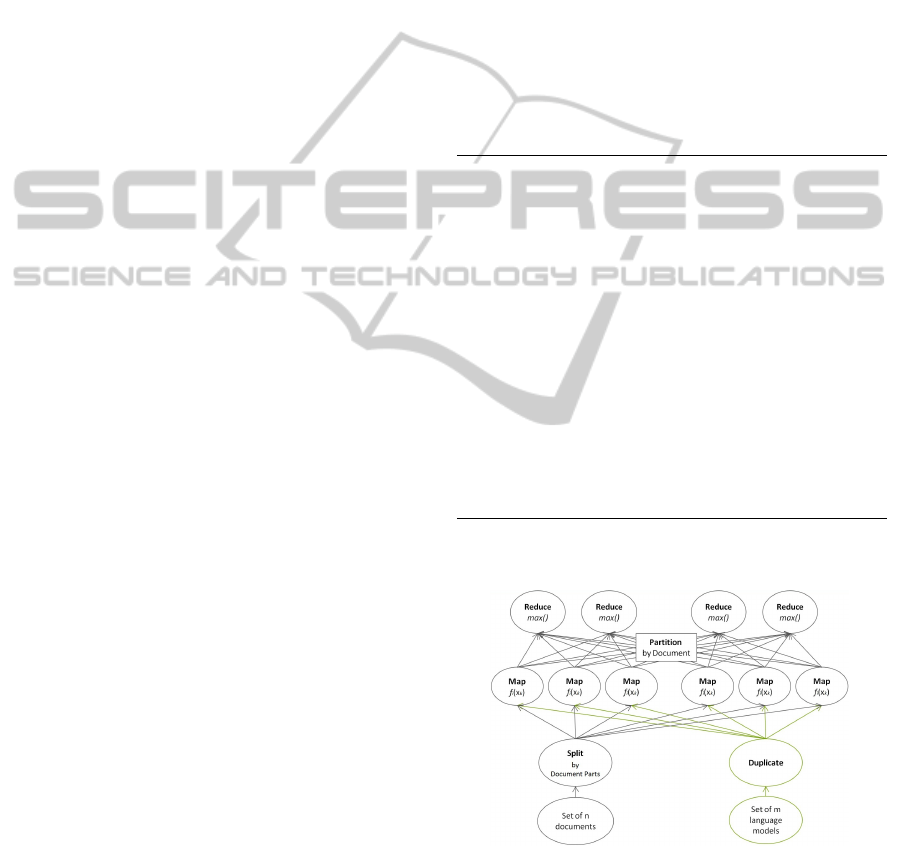
Figure 1: Dataflow for Script 2.
Even though the pseudo code denotes with
∑
,
∏
and max many obvious aggregation functions to be
chosen for multiple Reduce tasks, we kept the struc-
ture simple, for the sake of the example, and chose
only a single Map and a single Reduce task. As in
the training phase we have to get the statistics of a
AdvancedAnalyticswiththeSAPHANADatabase
63
document during the Map phase, but this time we do
not directly pass them to the Reduce task. Instead we
compare the statistic to the language models to calcu-
late the conditional probability P(l
j
|c
i
), which means
that each Map job has to have a copy of the language
models. The models must therefore be broadcast to
each Map task. To minimize the data transportation
between Map and Reduce tasks, it is advisable to cal-
culate the discriminate function in line 12 as part of
the Map job—or as an additional Combine task—and
leave the final class assignment with max to the Re-
duce task.
Figure 1 illustrates the MapReduce data flow of
the discussed naive Bayes classification.
Since the final assignment for the class (e.g., lan-
guage) has to be done centrally for each document,
the maximal number of parallel Reduce tasks is lim-
ited by the number of documents to be classified. The
degree of parallelization of the Map job however is
only limited by the combination of document parts
and classes, since each document part has to be com-
pared to each class. However if only few documents
and classes have to be considered, it may as well make
sense to separate the Map jobs further along different
features.
2.3 Repeated-pass
The class of iterative ML algorithms—perhaps the
most common within the machine learning research
community—can also be expressed within the frame-
work of MapReduce by chaining together multiple
MapReduce tasks (Chu et al., 2006). While such al-
gorithms vary widely in the type of operation they
perform on each datum (or pair of data) in a training
set, they share the common characteristic that a set of
parameters is matched to the data set via iterative im-
provement. The update to these parameters across it-
erations must again decompose into per-datum contri-
butions. The contribution to parameter updates from
each datum (the Map function) depends on the output
of the previous iteration.
When fitting model parameters via a perceptron,
boosting, or support vector machine algorithm for
classification or regression, the Map stage of train-
ing will involve computing inference over the train-
ing example given the current model parameters. A
subset of the parameters from the previous iteration
must be available for inference. However, the Re-
duce stage typically involves summing over parame-
ter changes. Thus, all relevant model parameters must
be broadcast to each Map task. In the case of a typ-
ical featurized setting, which often extracts hundreds
or thousands of features from each training example,
the relevant parameter space needed for inference can
be quite large.
01. do{
02. E-step: z
(m)
= argmax
z∈Z(x)
P(z|x,θ
(m)
) } MAP
03. M-step: θ
(m+1)
= argmax
θ∈Ω
P(x,z
(m)
|θ) } REDUCE
04. } while(θ
(m)
− θ
(m+1)
> ε) } BREAK
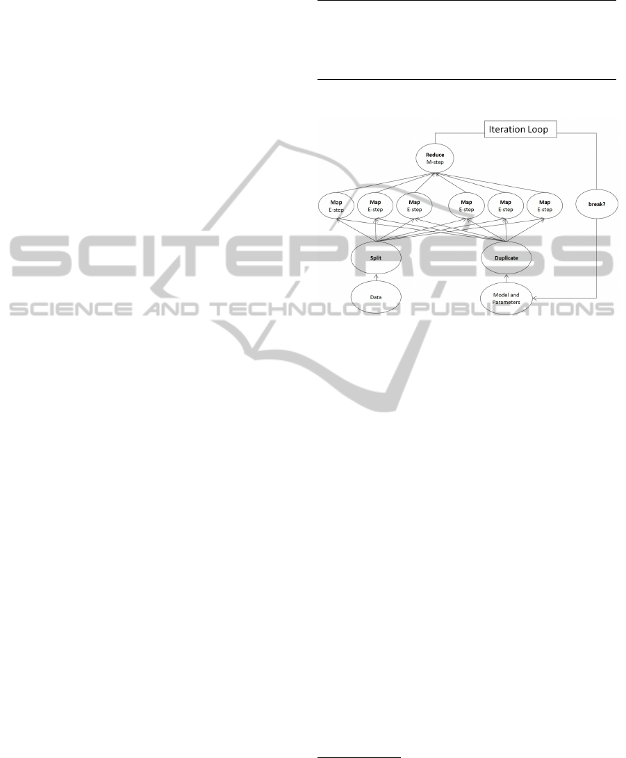
Script 3: Pseudo Code for the EM-Algorithm.
Figure 2: Dataflow for Script 3.
To illustrate this we return to our previous exam-
ple of Gaussian distributions to model language prop-
erties based on the letter distribution. In section 2.1
we kept things simple and described the letter distri-
bution of a single letter with a single Gaussian func-
tion defined by a single means and standard devia-
tions. This is a simplifying assumption commonly
found to be able to solve a given problem with the
first class of Single-pass algorithms. But in fact a sin-
gle Gaussian function may not be good enough to de-
scribe the observed letter distribution. We may have
to use a different distribution function or model like
a Gaussian mixture model (GMM), consisting of a
weighted combination of multiple Gaussian distribu-
tions. The problem here is that given the letter ob-
servations in our training data set, we can not deduce
multiple Gaussian distributions. We just would not
know which letter observation in which document has
to be associated with which distribution. But with-
out this knowledge we are not able to describe the
different Gaussian distributions in the first place, be-
cause we can not calculate the means and standard
deviations for the different distributions and in conse-
quence can not fit the GMM weights to describe the
observed distribution.
1
1
This is a classic situation where on the one hand latent
variables (the association of observation to distribution) are
missing, which would be needed to fit a optimized model.
But on the other hand to approximate the latent variables, a
model is missing to derive the variable from.
DATA2013-2ndInternationalConferenceonDataManagementTechnologiesandApplications
64

The well-known EM algorithm (A. P. Dempster,
2008) is an iterative approach to solve this kind of
situations, by maximizing the likelihood of a train-
ing set given a generative model with latent variables.
The pseudo code for the EM algorithm is shown in
script 3. The expectation step (E-step) of the algo-
rithm computes posterior distributions over the latent
variables z given the current model parameters θ
(m)
and the observed data x. The maximization step (M-
step) adjusts model parameters θ
m+1
to maximize the
likelihood of the data x assuming that latent variables
z
(m)
take on their expected values.
In our GMM example the aim of the EM-
algorithms is to estimate the unknown parameters rep-
resenting the mixing value τ
i
between the Gaussians
and the means µ
i
and standard deviations σ
i
with
θ = (τ
1
,τ
2
,µ
1
,µ
2
,σ
1
,σ
2
), based on the latent vari-
able z assigning each letter to one of two possible
Gaussian distributions. The naive representation of z
is a very high dimensional vector with an entry for
each single occurring letter in all documents. Ap-
proximating such a high dimensional vector may not
make sense, so a simplification could be to assume
that all letters of a document can be assigned to the
same Gaussian distribution. This assumption in par-
ticular does make sense, if we know that the docu-
ments used for the training task come from different
sources. For instance, some documents contain politi-
cal speeches, whereas others are taken from technical
reports, and we can therefore assume that the different
vocabulary in the documents influence different letter
distributions even within the same language.
Projecting onto the MapReduce framework (see
Figure 2), the Map task computes posterior distri-
butions over the latent variables of a datum using
the current model parameters; the maximization step
is performed as a single reduction, which sums the
statistics and normalizes them to produce updated pa-
rameters. This process has to be repeated until a break
condition is reached, which is usually defined by a de-
crease of model parameter modifications during the
iterations.
2.4 Cross Apply Repeated-pass
The previous sections 2.2 and 2.3 both discussed clas-
sic processing patterns found in common ML algo-
rithms, which are beyond the standard MapReduce
paradigm. Section 2.2 introduced the repeated but in-
dependent application of the same logic to variations
of data or models, whereas section 2.3 introduced the
repeated and dependent application of the same logic
in an iterative fashion. In many ML algorithms you
find only one of those pattern at a time, but in fact they
are orthogonal and can also appear both at the same
time. This combined pattern of repeated apply with
iterative learning can in particular be seen when ML
algorithms are combined, which is commonly done
in the field of machine learning. Often this pattern
can be mapped to a number of independent instances
of the iterative learning pattern, each processing its
iterative loop independently. But it is not always pos-
sible to keep the iterative loop on the outermost part
of the combined algorithm. In particular if a sepa-
ration between per-processing and loop processing is
unwanted.
01. for all classes c
i
∈ c
1
,...,c
m
02. for all documents d
k
∈ d
1
,...,d
n
of class c
i
03. for all feature l
j
∈ l
1
,...,l
v
of document d
k
04. sum
k
(l
j
) = count(l
j
);
05. od;
06. od;
MAP
1
07. for all feature l
j
∈ l
1
,...,l
v
in all d
k
of class c
i
08. x
j
=
S
n
k=1
sum
k
(l
j
) } RED
1
09. do{
10. z
(m)
j
= argmax
z∈Z(x
j
)
P(z
j
|x
j
,θ
(m)
j
) } MAP
2
11. θ
(m+1)
j
= argmax
θ∈Ω
P(x
j
,z
(m)
j
|θ
j
) } RED
2
12. } while (θ
(m)
j
− θ
(m+1)
j
> ε) } BRK
2
13. GMM
j
= θ
(m)
j
14. od;
15. M
i
=
S
v
j=1
GMM
j
} RED
3
16. od;
Script 4: Pseudo code to calculate GMM distributions for a
set of features and different classes.
To illustrate this we return to our previous ex-
ample. In section 2.3 we discussed how the EM-
Algorithm can be used to iteratively retrieve all re-
quired parameters for a Gaussian mixture model
(GMM) to describe a single letter distribution, but in
fact for our naive Bayes model we do not need a sin-
gle GMM, but one for each letter-class combination.
So for a GMM version of the naive Bayes model the
Pseudo code of script 1 in the lines 9-14 would have
to be replaced with the Pseudo code from script 3,
as denoted in script 4. Consequently the code part
(lines 7-16), that was before handled by a single Re-
duce task, now splits further apart into smaller tasks
including the Map/Reduce tasks and the loop of the
EM algorithm.
2.5 Summary
In the previous sections we introduced four machine
learning processing patterns. The first pattern ’Single-
pass’ had a very close match to the classic MapRe-
duce programming paradigm. Data is read once dur-
ing a single data pass in the Map phase and results
AdvancedAnalyticswiththeSAPHANADatabase
65
are combined and aggregated during a final Reduce
phase.
The second processing pattern ’Cross Apply’ ex-
tends the classic MapReduce paradigm such that more
than one data source (typically data and model) has
to be jointly processed and the cross combination of
both (data and model) spans the degree of parallel
processing.
The third pattern ’Repeated-pass’ further intro-
duces the data dependent loop. Again data can be pro-
cessed in parallel using Map and Reduce tasks, but the
process has to be iteratively repeated, typically with a
data dynamic break condition. Since classic MapRe-
duce frameworks do not provide a solution for loops,
this iterative loop has usually to be handled in an ap-
plication layer on top of the MapReduce framework.
Performance wise this kind of context switch is to be
avoided, but moreover it is only feasible if the loop is
at the outermost part of the algorithm.
Our fourth processing pattern ’Cross Apply
Repeated-pass’ however introduced loops as being
part of the parallel processing threads, where this is
not true anymore.
Additionally the fourth example clearly illustrates
that the algorithms in our examples demand more
flexible combinations of Map and Reduce tasks than
the ordinary closely coupled MapReduce. In fact we
find many examples of multiple Reduce tasks, per-
forming aggregations and preaggregations at differ-
ent stages of the algorithm, similar to discussion in
MapReduceMerge (Yang et al., 2007).
Already in our first example in script 1 the brack-
ets indicating a single Map followed by a single Re-
duce, are in fact a simplification. Having a closer look
at the pseudo code we see that the count(l
j
) Opera-
tion in line 4 is equivalent to the well known word
count example normally used to illustrate a classic
Map-Reduce task. Counting the features for docu-
ment parts and aggregating the count documentwise,
would be the usual MapReduce approach. But in
the context of our algorithm we thereby introduce a
MapReduceReduce. Having an even closer look at
the pseudo code we see that the union operation in
line 16 is again a decoupled Reduce (or merge) task,
which can be done independent and on top of the par-
allel calculated Gaussian distributions. So already
our first Script shows an example for MapReduce-
ReduceReduce rather then just MapReduce.
The text classification example of the previous
sections has been primarily chosen for illustration
purpose and because of its close relation to clas-
sic MapReduce tasks. Although text classification
applications usually do not require data schemas,
it is not uncommon that systems like Customer-
Relationship-Management indeed store text content
in a database. This is in particular the case for the
SAP HANA database, which has a text search origin.
Other machine learning algorithms, such as k-Means,
k-Nearest Neighbor and Support Vector Machines,
can benefit even more from being implemented in
a database context because of the support of data
schemas.
3 WORKER FARM
The goal of our architecture is to embed second-order
functions, such as Map and Reduce, as seamless as
possible into the otherwise relational concept of the
SAP HANA database. As such, we attempt to in-
clude custom code, written in non-relational program-
ming languages, such as R, into the parallelized exe-
cution plan of the database. As basic structure for
embedding second-order functions into the Database
we chose one of the most classical task parallel skele-
tons: the Worker Farm (Poldner and Kuchen, 2005).
The Worker Farm skeleton consists of the following
three basic methods.
Figure 3: The Worker Farm parallel architecture.
1. The split() method is responsible for distributing
the incoming dataset.
2. The work() method provides individual runtime
environments for each dataset executing the pro-
vided first-order function.
3. The merge() method combing the individual re-
sults from all workers.
Figure 3 illustrates the three methods and the run-
time behavior of the database including those meth-
ods as logical database operators.
Instead of operating on a key-value store orga-
nized through a distributed file system, the SAP
HANA database operates on in-memory tables orga-
nized through a distributed relational database sys-
DATA2013-2ndInternationalConferenceonDataManagementTechnologiesandApplications
66

tem. Consequently the methods split(), work() and
merge() operate on relational in-memory tables.
The split() method may for example implement
any kind of distribution and partitioning schema,
which guarantees for n following worker operations
n distinct in-memory tables references. This may be a
duplication of the input table by multiple reference,
this may be a partitioning of the input table using
hash, round-robin or range partitioning or even a cus-
tom partitioning provided through custom code.
The work() method is a placeholder for custom
code, provided though one of the custom code lan-
guages supported by the SAP HANA database, such
as R (R Development Core Team, 2005) or L.
Open source R is a very flexible and extension-rich
programing language particularly designed for ma-
chine learning and data mining tasks. R comes with
its own runtime, and input tables consumed by a cal-
culation Engine R operator (Große et al., 2011) are
copied to it for processing.
L is a SAP-internal, LLVM-based, just in time com-
piled programming language and provides a safe sub-
set of C/C++. L is statically typed and allows to define
and call functions, or use methods defined on SAP
HANA database objects, but it does not have unsafe
access to pointers. As such, an L operator allows to
directly manipulate in-memory tables provided as in-
put to the operator.
The merge() method finally combines the results
form all workers. The simplest and maybe most com-
mon merge method is a union all. But also any kind
of aggregation function or custom merge maybe used.
3.1 Stacked Worker Farm
In many cases of machine learning applications that
follow the Single-pass pattern (see section 2.1), a
single Worker Farm with an aggregation function as
merge()-method is sufficient to express the neces-
sary logic. For other cases, where custom coded Re-
duce tasks are required, stacking two or more Worker
Farms is necessary.
Multiple Worker Farm skeletons and their exe-
cuted custom code can be stacked on top of each other
in a way that the output of one Worker Farm will
be used as input to the next. Different from clas-
sic MapReduce frameworks, recurring Map or Re-
duce tasks do neither involve writing intermediate re-
sults to the file system nor jumping between applica-
tion layer and MapReduce framework for orchestra-
tion of repeated executions. Instead, intermediate re-
sults are kept as temporal in-memory tables (and only
persisted if explicitly enforced), and the orchestration
of repeated executions is handled inside the database
by building a unified plan, which can further be opti-
mized.
Depending on the used split and merge methods
and the involved list of key columns, the Optimizer
may choose to combine different Worker Farm layers
to a combined execution plan avoiding intermediate
steps. For instance, with an hash split and union all
merge, it is possible to exploit key/superkey relation-
ships and reuse partitioning done for the first Worker
Farm also for the second Worker Farm, or—as illus-
trated in figure 4—introduce a Shuffle step between
two Worker Farm layers instead of single point merge
and followed by another split. This is possible be-
cause the framework is—different to classic MapRe-
duce implementations—aware of key/superkey rela-
tionships since combined keys are not hidden from
the framework, but exposed by the list of key columns
used for the split-method.
Figure 4 illustrates four possible optimizations,
which result from four different relationships be-
tween the split criteria of the first Worker Farm s
1
and the second s
2
. The rightmost execution plan
shows the case where s
1
and s
2
are independent and
a repartitioning—in the context of MapReduce called
Shuffle—of the output of the first Worker Farm is re-
quired. From this figure we can see that the classic
Map-Shuffle-Reduce is just one possible outcome of
combining two Worker Farms.
Since our framework is embedded inside a
database we can not only stack multiple Worker
Farms, we can also combine a Worker Farm with a
relational operator like a Join. This is exactly what
is needed to implement the Cross Apply Pattern (see
section 2.2). Multiple Data Sources are combined
using a join operation followed by one or several
stacked Worker Farms. Depending on the relationship
of Worker Farm split and join conditions, the join op-
eration can be included into the parallel processing of
the Worker Farm.
3.2 Worker Farm Loop
In oder to support loops within the engine, we extend
the basic Worker Farm as illustrated in Figure 5.
The first extension is that the work methods con-
sume two distinct input sets. Invariant data and vari-
ant data, feed to the worker with possible two differ-
ent but compatible split methods. The main reason
to distinguish between the two different input sets is
the optimization that invariant data only has to be dis-
tributed once and can be kept in the cache, while vari-
ant data has to be distributed for each iteration.
A second extension is that the work method
may—but does not have to—return two distinct out-
AdvancedAnalyticswiththeSAPHANADatabase
67
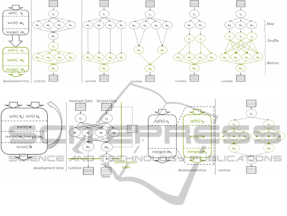
Figure 4: Stacking two Worker Farms.
Figure 5: The Worker Farm Loop.
put sets.
The most important extension however is the in-
troduction of a break() method. The break() method
is a placeholder for custom code, which consumes the
merge results m
2
of the worker and returns a boolean
indicating whether or not another iteration is to be
triggered. If no further iterations are to be trigged,
the results of the merge m
1
is returned, otherwise the
result if the merge m
2
is put to the cache and fed back
as variant data for the processing of another iteration.
An engine-internal orchestration layer is responsible
for keeping track of the cached in-memory tables and
to trigger further iterations.
With the extended Worker Farm Loop we are able
to express algorithms described with the processing
pattern Repeated-pass (see section 2.3).
3.3 Embedded Worker Farm
With the ability to handle loops inside the engine, as
discussed in previous section 3.2, we already fulfill an
imported requirement of our fourth processing pattern
’Cross Apply Repeated-pass’ (see section 2.4). How-
ever, missing is a construct to express loops as being
part of an otherwise parallel processed execution. For
this another extension of the Worker Farm skeleton is
required. The ability to embed a Worker Farm or a
Worker Farm Loop inside another Worker Farm. To
Figure 6: Worker Farm as part of another Worker Farm.
support this, we allow to reference another Worker
Farm in place of the work method. Figure 6 illus-
trates the embedding of a Worker Farm without Loop
as part of another Worker Farm.
4 EVALUATION
We have implemented the different Worker Farmer
Patterns within the SAP HANA database using the
calculation engine, which allows to define a database
execution plan by expressing it through an abstract
data flow graph (calculation model). Details regard-
ing calculation models can be found at (Große et al.,
2011). Source nodes represent either persistent table
structures or the outcome of the execution of other
calculation models. Inner nodes reflect the data pro-
cessing operations consuming either one or multiple
incoming data flows. Those data processing opera-
tions can be intrinsic database operations like pro-
jection, aggregation, union or join, but in our Map-
Reduce context more importantly they can also be
custom operators processing custom coding. With
this we can express Map and Reduce as well as any
other second-order function as custom operator, in-
troducing the actual data processing though custom
code.
In the following section we discuss our evalua-
DATA2013-2ndInternationalConferenceonDataManagementTechnologiesandApplications
68
tions for each of the discussed processing pattern. The
hardware used for our evaluation is an Intel
R
Xeon
R
X7560 processor (4 sockets) with 32 cores 2.27 GHz
using hyper-threading and 256 GB of main memory.
All experiments where conducted based on the Cana-
dian Hansard Corpus (The Canadian Hansard Corpus,
2001), a multilingual text corpus derived from debates
of the Canadian Parliament published in the country’s
official languages English and French.
4.1 Single-pass
For the evaluation of the Single-pass pattern (see sec-
tion 2.1) we extracted 994,475 text documents of
length 1000 characters from the Hansard Corpus and
implemented the naive Bayes Training example from
Script 1 using a Stacked Worker Farm (see section
3.1). The first Worker Farm (Map) implements the
character counting as indicated in Script 1 and par-
allelizes over the number of documents. The sec-
ond Worker Farm (Reduce) implements the mean and
standard deviation calculation, parallelizing over the
feature (26 letters) class (2 languages) combinations.
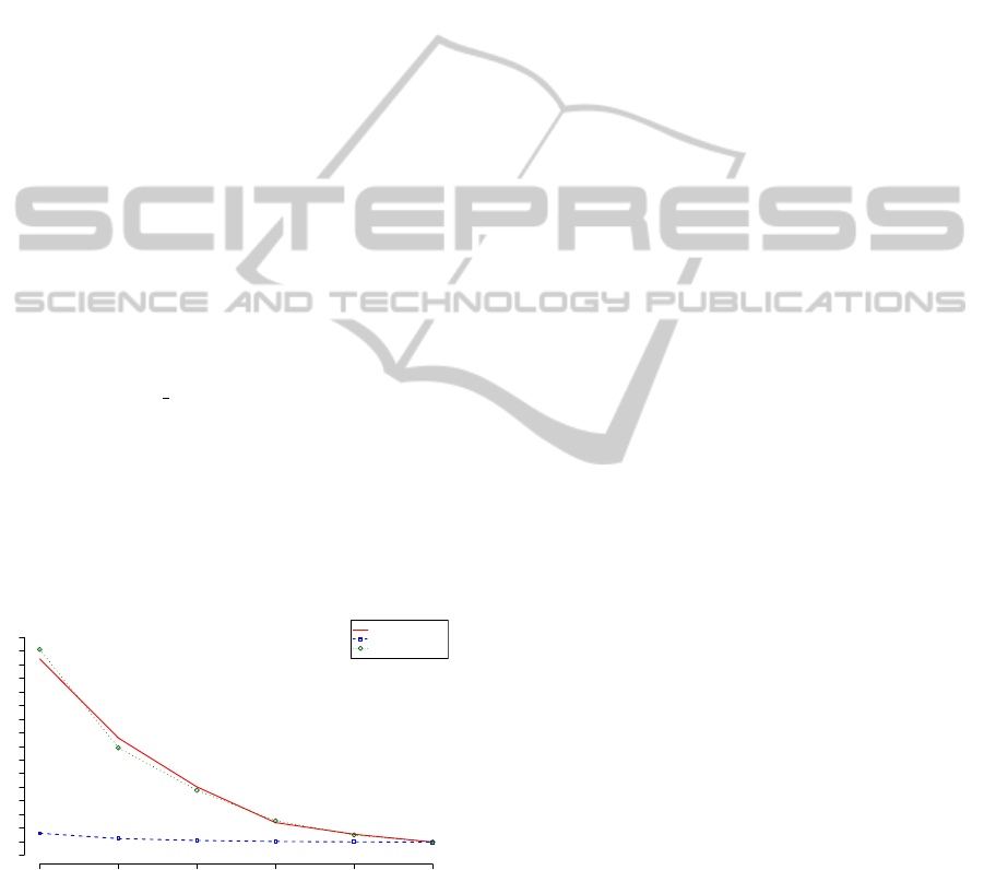
Figure 7 shows the actual execution time, when
varying the number of Map and Reduce tasks. The
curve label Map-X Reduce-32 for instance means
that the measurements we conducted were using a
constant number of 32 Reduce tasks and varying num-
ber of X Map tasks. It can easily be seen that the over-
all execution time is mainly dominated by the number
of Map jobs, whereas the Reduce task of calculating
mean and standard deviation does not scale, because
the calculation is just to simple too keep the CPUs
busy.
●
●
●
●
●
●
Number of Map/Reduce tasks
Execution time (seconds)
1 2 4 8 16 32
0 200 400 600 800 1000 1200 1400 1600
●
Map−X_Reduce−32
Map−32_Reduce−X
Map−X_Reduce−X
Figure 7: Execution time for naive Bayes Training.
4.2 Cross Apply
For the evaluation of the Cross Apply pattern (see sec-
tion 2.2) we implemented the Maximum-likelihood
classification example from Script 2 by stacking three
Worker Farms. The classification was conducted
based on 198,895 text documents of length 5000 char-
acters. The first Worker Farm (Map1) does the let-
ter counting analogous to the Map-task in the Train-
ing example, calculating the counting statistic for sub
documents of length 1000 characters. The second
Worker Farm (Map2) implements the actual classifi-
cation, comparing the sub document statistics against
each language model (letter mean and standard de-
viation trained during a previous evaluation) and as-
signing each sub document to a class. Both Map
tasks parallelize over the number of sub documents
and are therefore scheduled together building concep-
tional one joined Map-task. The third Worker Farm
(Reduce) however combines the sub document clas-
sification by majority voting and finally assigns each
document a class. It parallelizes over the original doc-
uments.
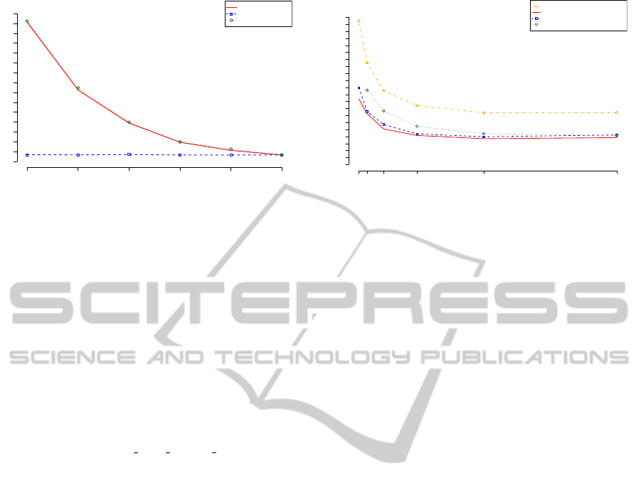
Figure 8 shows the execution time, when varying
the number of Map and Reduce tasks. As expected
the Map, doing both counting and actual classifica-
tion scales, whereas the Reduce doing only the the
final aggregation does not. Note the minimal increase
of the Reduce curve, indicating the overhead of the
system. It also shows that the saturation of the Map
curve is mainly caused by too few workload per CPU
and not by the systems overhead for scheduling the
tasks.
4.3 Repeated-pass
For the evaluation of the Repeated-pass pattern (see
section 2.3) we used the Worker Farm Loop skele-
ton from section 3.2 implementing a data flow sim-
ilar to figure 2. The evaluation was conducted us-
ing three datasets: 465,115 English (ENG) docu-
ments, 529,235 French (FRA) documents, and a su-
perset (ALL) containing both classes. Each of the
datasets had been preprocessed to extract the letter
counting. The E-Step (Map) calculates the distance
between each document and its 26 letter counts and 5
Gaussian distribution models per class with mean and
standard deviation for each letter, assigning the best
fitting model. The M-Step (Reduce) recalculates the
mean and standard deviation, given the assignment
from the E-Step. In this setup the EM-Algorithm is
not much different from a k-Means Clustering, except
that the overall goal is not the clustered documents but
the Gaussian models and the weights between them,
given by the distribution of documents to the models.
To guarantee comparable results between multiple ex-
ecutions we use a fixed number of ten iterations, in-
stead of a dynamic break condition.
The measurements in Figure 9 show a quick satu-
ration after already 8 parallel Map tasks and a slight
AdvancedAnalyticswiththeSAPHANADatabase
69
●
●
●
●
●
●
Number of Map/Reduce tasks
Execution time (seconds)
1 2 4 8 16 32
0 200 400 600 800 1000 1200 1400
●
Map−X_Reduce−32
Map−32_Reduce−X
Map−X_Reduce−X
Figure 8: Execution time for naive Bayes Classification.
increase between 16 to 32 map job due to the system
scheduling overhead. Furthermore we can see that the
execution time for the superset (ALL) is more or less
a direct aggregation of the execution times of the two
subsets (ENG and FRA).
4.4 Cross Apply Repeated-pass
We have argued in section 2.4 that the GMM model
fitting of the EM-Algorithmn for two or more classes
(FRA and ENG) contain two or more independent
loops, which can be modeled and executed as such.
The curve ”ParallelLoop ALL Map-X Reduce-2” in
Figure 9 shows the execution time for such indepen-
dent loops. We implemented it using an embedded
Worker Farm (see section 3.3) including two Worker
Farm Loops. The outer Worker Farm splits the data
into the two classes English and French, whereas the
inner embedded Worker Farm Loops implement the
EM-Algorithm, just like in previous Repeated-pass
evaluation.
The curve for the embedded parallel loops with p
Map tasks, corresponds to the two single loop curves
for FRA and ENG with p/2 Map tasks. As expected
we can see that the execution time of the embedded
parallel loop is dominated by the slowest of the in-
ner loops (here FRA). Nevertheless we can also see
that executing independent parallel loops is still faster
than one loop with multiple parallel Map tasks. This
is because even if we have multiple Map and Reduce
tasks, we still have for each loop iteration a single
synchronization point deciding about the break con-
dition.
5 RELATED WORK
Most related to our approach are extensions to
Hadoop to tackle its inefficiency of query processing
●
●
●
●
●
●
Number of Map tasks
Execution time (seconds)
1 2 4 8 16 32
0 40 80 120 160 200 240 280 320 360 400
●
SingleLoop_ALL_Map−X_Reduce−2
SingleLoop_ENG_Map−X_Reduce−1
SingleLoop_FRA_Map−X_Reduce−1
ParallelLoop_ALL_Map−X_Reduce−2
Figure 9: Execution time for EM-Algorithm (Script 3).
in different areas, such as new architectures for big
data analytics, new execution and programming mod-
els, as well as integrated systems to combine MapRe-
duce and databases.
An example from the field of new architectures is
HadoopDB (Abouzeid et al., 2009), which turns the
slave nodes of Hadoop into single-node database in-
stances. However, HadoopDB relies on Hadoop as its
major execution environment (i.e., cross-node joins
are often compiled into inefficient Map and Reduce
operations).
Hadoop++ (Dittrich et al., 2010) and Clydes-
dale (Kaldewey et al., 2012) are two examples out
of many systems trying to address the shortcomings
of Hadoop, by adding better support for structured
data, indexes and joins. However, like other sys-
tems, Hadoop++ and Clydesdale cannot overcome
Hadoop’s inherent limitations (e.g., not being able to
execute joins natively).
PACT (Alexandrov et al., 2010) suggest new ex-
ecution models, which provide a richer set of opera-
tions then MapReduce (i.e., not only two unary oper-
ators) in order to deal with the inefficiency of express-
ing complex analytical tasks in MapReduce. PACT’s
description of second-order functions with pre- and
post-conditions is similar to our Worker Farm skele-
ton with split() and merge() methods. However, our
approach explores a different design, by focusing on
existing database and novel query optimization tech-
niques.
HaLoop (Bu et al., 2010) extends Hadoop with
iterative analytical task and particular addresses the
third processing pattern ’Repeated-pass’ (see section
2.3). The approach improves Hadoop by certain op-
timizations (e.g., caching loop invariants instead of
producing them multiple times). This is similar to our
own approach to address the ’Repeated-pass’ process-
ing pattern. The main difference is that our frame-
work is based on a database system and the iteration
handling is explicitly applied during the optimization
DATA2013-2ndInternationalConferenceonDataManagementTechnologiesandApplications
70

phase, rather then implicitly hidden in the execution
model (by caching).
Finally, major database vendors currently include
Hadoop as a system into their software stack and
optimize the data transfer between the database and
Hadoop e.g., to call MapReduce tasks from SQL
queries. Greenplum and Oracle (Su and Swart, 2012)
are two commercial database products for analytical
query processing that support MapReduce natively in
their execution model. However, to our knowledge
they do not support extensions based on the process-
ing patterns described in this paper.
6 CONCLUSIONS
In this paper we derived four basic parallel processing
patterns found in advanced analytic applications—
e.g., algorithms from the field of Data Mining
and Machine Learning—and discussed them in the
context of the classic MapReduce programming
paradigm.
We have shown that the introduced programming
skeletons based on the Worker Farm yield expres-
siveness beyond the classic MapReduce paradigm.
They allow using all four discussed processing pat-
terns within a relational database. As a consequence,
advanced analytic applications can be executed di-
rectly on business data situated in the SAP HANA
database, exploiting the parallel processing power of
the database for first-order functions and custom code
operations.
In future we plan to investigate and evaluate op-
timizations which can be applied combining classical
database operations - such as aggregations and joins -
with parallelized custom code operations and the lim-
itations which arise with it.
REFERENCES
A. P. Dempster, N. M. Laird, D. B. R. (2008). Maxi-
mum Likelihood from Incomplete Data via the EM
Algorithm. Journal of the Royal Statistical Society,
39(1):1–38.
Abouzeid, A., Bajda-Pawlikowski, K., Abadi, D., Silber-
schatz, A., and Rasin, A. (2009). HadoopDB: an
architectural hybrid of MapReduce and DBMS tech-
nologies for analytical workloads. Proc. VLDB En-
dow., 2(1):922–933.
Alexandrov, A., Battr
´
e, D., Ewen, S., Heimel, M., Hueske,
F., Kao, O., Markl, V., Nijkamp, E., and Warneke, D.
(2010). Massively Parallel Data Analysis with PACTs
on Nephele. PVLDB, 3(2):1625–1628.
Apache Mahout (2013). http://mahout.apache.org/.
Bu, Y., Howe, B., Balazinska, M., and Ernst, M. D. (2010).
HaLoop: Efficient Iterative Data Processing on Large
Clusters. PVLDB, 3(1):285–296.
Chu, C.-T., Kim, S. K., Lin, Y.-A., Yu, Y., Bradski, G. R.,
Ng, A. Y., and Olukotun, K. (2006). Map-Reduce for
Machine Learning on Multicore. In NIPS, pages 281–
288.
Dean, J. and Ghemawat, S. (2004). MapReduce: Simplified
Data Processing on Large Clusters. In OSDI, pages
137–150.
Dittrich, J., Quian
´
e-Ruiz, J.-A., Jindal, A., Kargin, Y., Setty,
V., and Schad, J. (2010). Hadoop++: making a yellow
elephant run like a cheetah (without it even noticing).
Proc. VLDB Endow., 3(1-2):515–529.
Gillick, D., Faria, A., and Denero, J. (2006). MapReduce:
Distributed Computing for Machine Learning.
Große, P., Lehner, W., Weichert, T., F
¨
arber, F., and Li, W.-
S. (2011). Bridging Two Worlds with RICE Integrat-
ing R into the SAP In-Memory Computing Engine.
PVLDB, 4(12):1307–1317.
Kaldewey, T., Shekita, E. J., and Tata, S. (2012). Clydes-
dale: structured data processing on MapReduce. In
Proc. Extending Database Technology, EDBT ’12,
pages 15–25, New York, NY, USA. ACM.
Poldner, M. and Kuchen, H. (2005). On implementing the
farm skeleton. In Proc. Workshop HLPP 2005.
R Development Core Team (2005). R: A Language and
Environment for Statistical Computing. R Foundation
for Statistical Computing, Vienna, Austria. ISBN 3-
900051-07-0.
Sikka, V., F
¨
arber, F., Lehner, W., Cha, S. K., Peh, T., and
Bornh
¨
ovd, C. (2012). Efficient transaction processing
in SAP HANA database: the end of a column store
myth. In Proc. SIGMOD, SIGMOD ’12, pages 731–
742, New York, NY, USA. ACM.
Su, X. and Swart, G. (2012). Oracle in-database Hadoop:
when MapReduce meets RDBMS. In Proc. SIGMOD,
SIGMOD ’12, pages 779–790, New York, NY, USA.
ACM.
The Canadian Hansard Corpus (2001). http://www.isi.edu/
natural-language/download/hansard.
Yang, H.-c., Dasdan, A., Hsiao, R.-L., and Parker, D. S.
(2007). Map-Reduce-Merge: simplified relational
data processing on large clusters. In Proc. SIGMOD,
SIGMOD ’07, pages 1029–1040, New York, NY,
USA. ACM.
AdvancedAnalyticswiththeSAPHANADatabase
71
