Performance Optimization in Intelligent Manufacturing

Decision Support System for Value Engineering in Flour Mills

Jürg P. Keller

and Mukul Agarwal

Institute for Automation, University of Applied Sciences and Arts Northwestern Switzerland,

Steinackerstrasse 5, 5210 Brugg-Windisch, Switzerland

Corporate Technology, Bühler AG, 9240 Uzwil, Switzerland

Keywords: Decision Support Systems, Intelligent Manufacturing, Systems Modelling and Simulation, Discrete-event

Systems, Supply Chain and Logistics Engineering, Production Planning, Quality Control and Management,

Performance Evaluation and Optimization, Human-system Interface, Cost and Value Engineering.

Abstract: The performance of modern flour mills depends crucially on value-engineering decisions involving optimal

mixing of up to 80 intermediate product streams into at most 6 final product streams during continuous

operation. Optimal mixing decision depends on given physical properties and yields of intermediate

streams, goals and constraints on physical properties and yields of final streams, physical and quality

constraints on mixing decision variables, and qualitative judgments relating value of final streams to their

physical properties. In a previous work, the authors presented an interactive tool that guided the production

personnel towards an optimal decision for fractions of each intermediate stream that should be piped to each

final stream. This tool could exploit multiple Linear Programming computations and graphic user-interface

to enable scenario overview and manoeuvring with no perceptible time lag. However, it cannot be used in a

majority of flour mills where each intermediate stream is diverted to a single final stream using physical

flaps. The mixed-integer programming required in this case renders the tool too slow for interactive use. In

this work, a new tool is developed for the prevalent case of discrete decision variables, which enables

computations and graphic interface for scenario manoeuvring without prohibitive time lag.

1 INTRODUCTION

Modern flour mills usually process a mixture of

different wheat grains through about a dozen

processing stages connected in series and parallel. In

each stage, grain particles are ground further and the

resulting particles are separated into various streams,

some of which go on to further processing stages

while some others are withdrawn as intermediate

product streams. This generates about 30 – 80

intermediate streams with different physical

properties and yields. These intermediate product

streams are mixed in continuous operation to

generate a mere 4 – 6 final product streams, which

are stored in product silos and then packed for

shipping.

The decision, how to mix the many intermediate

streams into a few product streams, is crucial for

generation of maximal sales value while accounting

for many constraints on the physical properties and

yields of the final streams, as well as on the mixing

decision variables. Since usually the sales value of

the final streams is not known as a function of their

physical properties, but can only be judged

qualitatively by the production personnel, tools are

needed to guide the decision process by showing

overviews of the compromises involved in the

various scenarios and letting decisions be made

successively and iteratively for each final stream.

This involves prolonged interactive use of the tool

until the final decision is reached. The tool must

therefore not only offer an intuitive and convenient

graphic interface, but also be computationally fast in

order to show scenario overviews and to allow

manoeuvring through scenarios without debilitating

time lag.

In a previous work (Keller and Agarwal, 2012),

the authors presented a tool that solved the above

challenges and was successfully tested in a real flour

mill. The tool dealt with the computational speed by

using multiple Linear Programming optimizations

implemented with an accelerated algorithm.

495

Keller J. and Agarwal M..

Performance Optimization in Intelligent Manufacturing - Decision Support System for Value Engineering in Flour Mills.

DOI: 10.5220/0004431204950504

In Proceedings of the 10th International Conference on Informatics in Control, Automation and Robotics (ICINCO-2013), pages 495-504

ISBN: 978-989-8565-71-6

 2013 SCITEPRESS (Science and Technology Publications, Lda.)

However, this solution is not applicable to a majority

of flour mills where each intermediate stream is

completely diverted to a single final stream, and no

splitting of an intermediate stream to multiple final

streams is possible due to constraints of the physical

flaps installed in the piping. In this work, therefore,

a new tool is developed for the situation involving

integer mixing-decision variables.

For the mixed-integer programming problem at

hand, many well-known algorithms already exist, in

principle. Some of these algorithms are summarized

in Chen et al. (2010). Employing these algorithms to

the problem at hand would mean optimizing up to

480 binary variables (for upto 80 intermediate

streams multiplied by up to 6 final streams). Since,

for binary variables, the Linear Programming

algorithm must be coupled with a Branch-and-

Bound procedure, this high number of binary

variables involves prohibitive computational time.

To circumvent this drawback, the problem is solved

here not for all final streams together, but for one

final stream at a time. This decoupling is feasible

and sensible for the problem at hand, because the

production personnel needs to specify physical-

property constraints for each final stream, and

prefers to do this only by specifying them (and

obtaining results) for one final stream at a time,

starting with the most valuable final stream.

Solving the decoupled problem for one single

final stream is similar to the problem addressed in

recent literature for distributed power-network

operation (Borghetti et al., 2011). The latter,

however, deals only with power as a single “physical

property” and with a-priori known, fixed constraints

for this physical property, whereas the problem at

hand involves up to 6 different physical properties,

and, more importantly, their constraints are not

known and cannot be specified a priori. The main

special feature of the problem at hand is that the user

needs to see the Pareto-optimal solution for all

possible physical-property constraints, so that he can

specify (actually, select) the constraints in an

informed manner, knowing the feasibility and the

influence of his choice on the final solution.

Precisely this special feature makes the use of

existing solutions computationally prohibitive for

the current problem. Computing and displaying all

binary solutions for the entire range of physical-

property constraints would be extremely time

consuming. To circumvent this issue, a new solution

strategy is used in this work that presents to the user

not the binary solutions, but instead a continuous-

solution space for the entire range of constraints.

Computation of the continuous-solution space

involves only Linear Programming, but no Branch-

and-Bound procedure, and is consequently fast. The

user can then conveniently analyse the solution

space and specify a (usually much narrower) range

of feasible constraints that she wants to focus on.

The solution procedure then generates all binary

solutions in the vicinity of the continuous solution.

The new tool circumvents the prohibitive

computational burden for the mixed-integer

programming problem by dividing the problem into

several sub-problems, by exploiting the continuous-

decision-variable solution as an anchor, and by using

an efficient procedure that employs Linear

Programming and Branch-and-Bound methods

intermittently to obtain binary solutions in the

vicinity of the anchor. A special graphic interface is

additionally designed to present flexible overviews

of resulting scenarios to the user. The new tool

allows fast, interactive decision making for the

considerably more challenging situation of discrete

decision variables. The tool was tested successfully

on real plant data.

2 PROBLEM FORMULATION

The production personnel in modern flour mills is

faced with, among others, the following crucial

decision. For each of the 30 – 80 intermediate

product streams withdrawn continuously from the

mill, the personnel has to decide, which of the 4 – 6

final product streams it should be diverted to. In a

majority of flour mills, this is an integer decision

that can take up to 6 values for each intermediate

stream (see Fig. 1).

The following facts render this decision difficult.

All intermediate and final streams are characterized

by identical physical quality parameters, 4 – 6 in

number. These properties are independent of each

other. Each property “mixes” linearly with respect to

the weight fractions. The yields (or flow rates) and

the physical properties of the intermediate streams

are given, whereas those of the final streams depend

on the decision and are subject to various

constraints. For example, a particular final stream

may represent a high-purity flour constrained by an

upper limit on the physical property “ash content”.

Another final stream may have a low yield limit due

to an already known sales to a particular customer,

or a high yield limit due to physical limitations of

piping, silo, or inventory. In addition, the flaps used

to divert an intermediate stream to a particular final

stream may have limitations in that a flap can

physically output only to certain final streams or

ICINCO2013-10thInternationalConferenceonInformaticsinControl,AutomationandRobotics

496

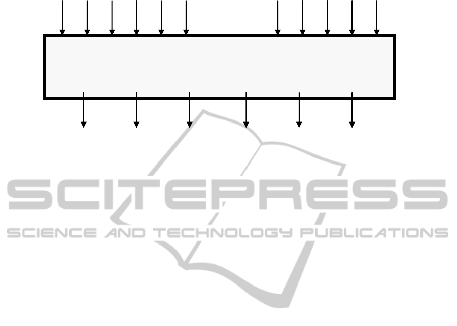
Figure 1: The decision problem.

quality constraints forbid it to output to certain final

streams. The decisions for all intermediate streams,

all final streams, all physical properties, and all

yields are interconnected in a complex way.

The decision making is complicated further by

the fact that, ultimately, the final streams should

have the highest possible sales value, but

characterization of this value is elusive, since the

function relating the sales price to the physical

properties is not fixed, or at least not known. The

user can only judge this value in a qualitative,

comparative way.

Obviously it is not possible even for an expert

personnel to make this decision in a near optimum

way. The decision is therefore usually determined by

on-line trial-and-error based on experience. It is far

from trivial to develop an appropriate decision-

support tool for this decision, since the tool must

optimize possible solutions for the entire range of

goal specifications, present all options and

compromises to the decision-maker in facilitating

overviews allowing for multiple dimensions,

conserve maximum flexibility for further steps while

making decisions in a particular step, and recompute

and redisplay all outputs without prohibitive time lag

when any user-input is changed.

A tool for supporting the above decision faces

several challenges.

1. Qualitative Judgement of Value: Since the value

of flours cannot be formulated explicitly as a

function of the flour properties and yields, a

decision-support tool cannot simply output a

unique optimal answer. Instead, the tool must

present all non-inferior outcomes and

compromises.

2. High Dimensional Space: Since large numbers

of properties, yields, intermediate streams and

final streams are involved in the decision-

making, the resulting high dimensionality is

challenging for the tool not only

computationally, but also in view of the 2D

graphic interface.

3. Need for Quick Reaction: The entire decision-

making with the support of the tool involves

scores of clicks and inputs from the user, while

each time the user appraises the tool output

before making the next click or input. The tool

must therefore respond within 15 – 20 seconds

after each click or input, so that the new result is

quickly visible for appraisal. Even then, the user

needs dozens of minutes of interactive use to

arrive at the complete final solution.

3 SOLUTION PROCEDURE

In principle, for the given problem, the tool must

calculate and display all discrete non-inferior

solution points, covering all intermediate and final

streams simultaneously. This is a formidable task

that would require unimaginably high computation

time, even using super computers.

3.1 Solution Strategy

A new solution strategy is developed that avails

itself of several accelerating improvements, so as to

achieve computation times of 15 – 20 seconds for

displaying the needed results.

Decision:

Each intermediate stream should be directed to which final stream?

Goal:

Maximize final stream value under a-priori unknown constraints.

_ _ _ _ _ _

30 – 80 intermediate streams with known properties & yields.

4 – 6 final streams with a-priori unknown properties and yields

that are determined interactively between the user and the tool.

PerformanceOptimizationinIntelligentManufacturing-DecisionSupportSystemforValueEngineeringinFlourMills

497

3.1.1 Stepwise Decision for each Final

Stream

The decision in the above mixed-integer problem

involves up to 80 decision variables (one for each

intermediate stream), each of which can take up to 6

discrete values (one for each final stream). The

mixed-integer problem is broken down to up to 6

sub-problems (one for each final stream). In each

sub-problem, each of the up to 80 decision variables

can take only 2 discrete values (yes/no, indicating

whether that intermediate stream is directed to the

sub-problem final stream or not). The massively

complex mixed-integer problem is thus reduced to a

few much simpler, mutually decoupled binary

problems. The consequence of this reduction is that

the decisions for each final stream can be made only

successively, and not all at once.

It turns out that, as in the previous work (Keller

and Agarwal, 2012), this poses no limitation for the

user, but is indeed in line with what the user would

prefer anyway. Due to the complexity of the given

problem, the user cannot simultaneously make

decisions for all final streams, even with the help of

a tool. The decision-making is therefore preferably

performed in steps, one step for each final stream,

usually beginning with the most valuable flour

stream and ending with the least valuable. The above

problem reduction allows the user to make a step

decision based on the results of previous step

decisions, as well as to revert to and re-adjust a

previous step decision.

3.1.2 Continuous Solution as Anchor

Even for a reduced sub-problem (for a single final

stream) as stated above, the number of possible

combinations of all binary decision variables is

formidably large. Computing all non-inferior

combinations for a sub-problem is therefore not

practical. A further insight into the problem leads to

a considerable relief in this respect.

Even a cursory reflection of the problem reveals

that the final solution of the binary-variable problem

must lie close to the solution of the continuous-

variable problem in the decision-variable space. This

holds not only from the process point-of-view, but

also from the viewpoint of the user. From the

process aspect, a unique optimal solution does not

even exist a priori, since the judgment of “value” is

merely qualitative and comparative, but not

absolute, i.e. the “optimal” solution is essentially

chosen by the user as a best-judged compromise.

From the user viewpoint as well, it is easier to first

“choose” a continuous solution, and then choose an

implementable binary solution in its vicinity.

The solution strategy thus lets the user first select

a sub-problem solution in the continuous space, as in

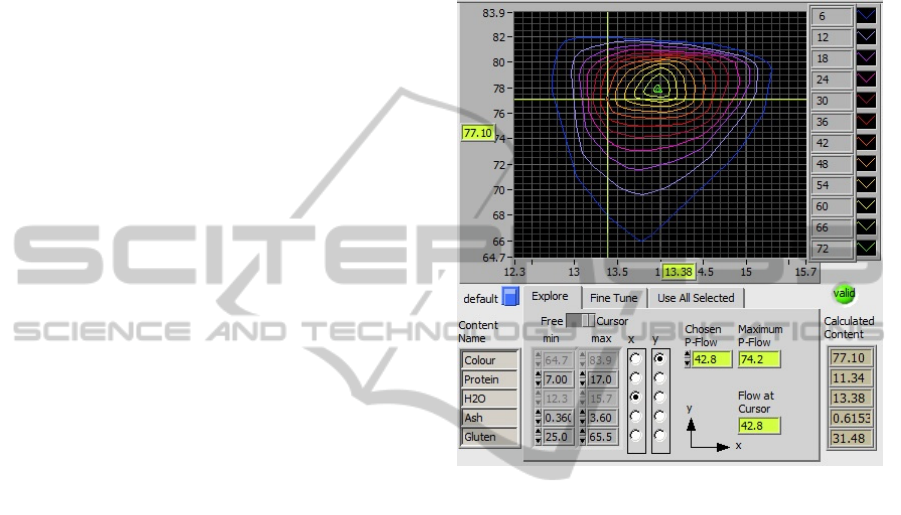
the previous work (Keller and Agarwal, 2012). Fig.

2 shows an example selection from the previous

work.

Figure 2: An example of the selection of a solution point

by the user in the continuous decision space (Keller and

Agarwal, 2012). (Figures 2 and 4 show realistically

created artificial data for illustration, since the actual

industrial data used for the tests is classified.)

The solution strategy in the current work thus

can use the selected point in the continuous space as

an anchor, and needs to merely compute all non-

inferior binary solutions in a reasonable vicinity of

this point. The computational burden is reduced

considerably through this anchoring, but is still

exorbitant.

3.1.3 Linear Programming with Relaxation

and Branch-and-Bound

The problem of finding binary solution points in the

vicinity of the continuous solution anchor point is

not amenable to Linear Programming (LP) solely,

since the latter delivers continuous values for the

decision variables. Finding binary points in the

vicinity would involve setting each continuous-value

decision variable to either 0% or 100%. This gives a

set of branches, for each of which another LP

problem with fewer decision variables is solved. The

ICINCO2013-10thInternationalConferenceonInformaticsinControl,AutomationandRobotics

498

branches with significantly poorer result than the

anchor are terminated, and in the remaining

branches the decision variables with continuous

values are set again to 0% and 100%, creating the

next set of combinatorial branches. This Branch-

and-Bound procedure, coupled with an LP solution

at each branch, and subsequent reduction in the

number of decision variables in each branching

stage, is repeated until no more branches are left.

The above procedure is still computationally

prohibitive, since the LP solutions at each branch

continue to involve a large number of decision

variables with continuous values. This large number

represents the number of basic variables in the LP

problem and equals the number of properties

involved plus one yield (i.e. up to 7). The solution

strategy therefore resorts to a relaxation method that

introduces auxiliary relaxation variables that can

take continuous values by becoming basic variables,

thereby relieving (at least) a corresponding number

of decision variables, which in turn become non-

basic, take a discrete 0-or-1 value, and lead to no

new branches. In practice, it was noticed that, when

yield is included as a relaxation variable, a

significantly higher number of decision variables is

“relieved” in this way, since not only the auxiliary

relaxation variables, but also several other auxiliary

variables in the LP formulation then become basic

variables.

The relaxation can be introduced for yield and/or

property variables, and allows that the value of these

variables in the anchor can be violated to a certain

extent. This “extent” can be specified with certain

weights, which could be optimized or selected by

trial-and-error. Two cases were tried in this work:

relaxation of yield only, and relaxation of yield as

well as all properties. In the first case, the relaxation

weights could easily be set by trial-and-error, since

their value is not very sensitive with respect to the

final result. In the latter case, however, setting the

relaxation weights for the properties is much more

difficult, not only because of the higher number of

coupled weights involved, but more so because the

choice of these weights is extremely sensitive with

respect to the final result. This solution avenue was

therefore dropped in favour of relaxation only with

respect to yield.

The above relaxation procedure is a variation of

the relaxation methods reported in the literature

(Guan et al., 2003; Lee et al., 2009). In these

methods, the Lagrangian relaxation weights serve to

penalize the constraint violation, i.e. for the problem

at hand, it would penalize the deviation of the yield

and property values from the anchor values. In the

procedure used above, the relaxation weights serve

to reduce the number of decision variables that come

out to be basic variables and consequently lead to

new branches.

3.2 Definitions

number of intermediate streams

number of final streams

number of properties

index for intermediate streams

index for final streams

index for properties

cost of i-th intermediate stream

weighting factor for scaling of k-th

property

i,p

yield of i-th intermediate stream that is

directed to the p-th final stream

i,max

maximum yield of i-th intermediate

stream that is available

yield of p-th final stream

increment for p-th final stream

k,i

weight fraction of k-th property in the

i-th intermediate stream

k,p

weight fraction of k-th property in the

p-th final stream

weight fraction of properties in P

p,d

matrix to select streams optimized

using LP in the mixed-integer problem

matrix to select streams with fixed

given values that are not optimized

number of streams with fixed given

values that are not optimized

vector with fixed given values for

streams selected using

(0 = not used, 1 = used)

fraction of a selected stream,





z0,1

with 0 = not used and 1 = used.

PerformanceOptimizationinIntelligentManufacturing-DecisionSupportSystemforValueEngineeringinFlourMills

499

In addition, let:











k,i w F

k,p k p P k,p k

pi,pF

Ww,nn

X x ,n n ,X x ,n 1

FF,n1

111 1,m1







 



 









(1)

3.3 LP Formulation for Splittable

Intermediate Streams

For the p-th final stream, the basic LP-problem with

splittable intermediate streams can be formulated as

follows:



ppp

np p

p,i i,max

ip,i

WF X P

1F P

als Matrix : F

0F F ,i

JcF

F: argmaxJF













 







(2)

Here, the objective function J is represented as a cost

criterion for intermediate streams. The cost factors c

can thereby represent either actual costs of these

flours or the strength of the user's a-priori

preference for wanting to use a particular

intermediate stream.

ik,pk,ik

cxwr







(3)

The above formulation is completely defined and

solvable when the yields and properties of the final

streams are predefined. But as mentioned above, this

is not the case here.

For the mixed-integer optimization in the present

situation, it is necessary to redefine the LP

formulation such that intermediate streams that are

predefined to be zero or F

i,max

get removed a priori.



p,r r p

,f f p

FSF

FSVF



 

(4)

Here S

selects streams that can be varied in the

range 0 to F

i,max

, and S

selects streams that are set

to 0 or F

i,max

depending on the value 0 or 1 in the

vector V. The LP formulation then becomes:



F,r F,f

rPn p,minp ff max

npnfmax

p,i i,max

pp,max

ip,i

rp p rp p

WS PI X P WS S V F

10 P1SVF

0F F ,i

0X X

JcF

SF X : argmaxJ SF X



















 





 



 













(5)

or in matrix form:



F,r

F,f

pn f max

rPn

p,min p f f max

p,i i,max

pp,max

ip,i

pp pp

P1 SVF

WS P I

XPWSSVF

0F F ,i

0X X

JcF

FX:argmaxJFX





































 





 



 











(6)

3.4 LP Formulation with Relaxation

The above formulation now needs to be modified to

include relaxation for yield, so as to force the

streams to be close to 0 or 100% of the intermediate

stream yield (see section 3.1.3). This is achieved by

allowing certain tolerances in the constraints. From

LP perspective, this creates additional basic

variables, such that the streams will take only

discrete values at either the upper or the lower

bound. For this purpose, define:

= z

i,max

pp,sollp, p,

PP P P







(7)

where P

p,soll

represents a given minimal yield that

must be reached and P

p,+

and P

p,-

represent relatively

small corrections to it. The latter appear in the

formulation as products with the property weight

fractions, leading to a bilinear optimization problem.

In order to avoid this bilinearity, the property weight

fractions in these cross-terms should be fixed. This

can be achieved by iterating the values of the

property weight fractions starting from the anchor

value.

The following LP formulation then results:

ICINCO2013-10thInternationalConferenceonInformaticsinControl,AutomationandRobotics

500



max F,f

T T

max,diag r P,soll n d d p, min p,soll f f max

rp,sollnfmax

pf p,max

p, max p, m

WF S P I X X X P WS S V F

FS 0 11 P 1 S VF

0z 1,i

0X X

0P P,0P P

















  

























 













i i,max F, p, F, p,

r p p, p, r p p, p,

JczF P P

S z X P P : arg max J S z X P P

 



 

   











(8)

or in matrix form:



F,fmax

p,min n f maxr

max,diag r P, min n d

p, min p , min f f max

p f p, max

p,d max

max r F, F ,

P1SVFFS 0 1

WF S P I X

XP WSSVF

0z1,i

0X X

0P P

JcFS0



















   

















































max m m

rpp,p,

cF SSz

S z X P P : arg max J

























(9)

3.5 Mixed-Integer Procedure for

Non-Splittable Intermediate

Streams

In the proposed solution procedure for the mixed-

integer problem at hand, the solution to the LP

problem in Eq. 9 is taken as the anchor starting point

to search for binary variable solutions in its vicinity.

The above LP problem comprises n

+3 equations

and n

-n

+2 variables that determine the split of the

intermediate streams. The chosen form for the

solution of this LP problem generates additional

+3 auxiliary variables based on the number of

equations. When the LP problem has been solved,

out of all variables precisely n

+3 variables emerge

as basic variables and take values that do not lie on

the constraints. If one of these n

+3 basic variables

belongs to the set z

, then the corresponding

intermediate stream gets split.

Since this split is not acceptable for the mixed-

integer problem at hand, a combination with the

Branch-and-Bound method is used. Branch-and-

Bound methods have a long history (Lawler and

Wood, 1966) for solving mixed-integer problems not

only in conjunction with Linear Programming using,

e.g., rules (Hansen et al., 1992) or heuristics

(Wolsey, 1980), but also for quadratic (Vielma et al.,

2008) and nonlinear (Leyffer, 2001) problems.

Using the Branch-and-Bound method for the

problem at hand, when one or more of the n

+3 basic

variables belong to the set z

, then several new LP

problems are generated using all possible integer-

value (0 or 1) combinations as a-priori fixed values

of these variables. All these LP problems are then

solved, and those branches are discarded that lead to

a considerably poorer objective-function value than

the source-branch LP solution. Generation of further

LP problems with new branching ends when all

branches get discarded.

3.6 Formal Solution Procedure

The above procedure is formalized as follows.

Analogous to the definition of S

and S

, define I

and I

as sets of indices for streams that are

optimized and that are fixed, respectively, and I as

the set of indices for all streams. Define

corresponding vectors z

and z

indicating fractions

of the intermediate stream that go into a final stream.

The vector z

containing fixed streams thus only

comprises values 0 and 1, whereas the vector z

starts out with real values and approaches the values

0 or 1 during the optimization.

Let the kth mixed-integer LP problem, LP

m,k

determine z

, I

, and the objective function value as:

r,k

, I

r,k

, J

m,k

)

= LP

m,k

f,k

, I

f,k

)

In the resulting vector z

r,k

, the indices for which the

value is not 0 or 1 form an index set I

r,k

. Next, all

(0,1)-combinations are determined for each z

r,k,i

with

i  I

r,k

. This generates a set of vectors Z

p,k

that must

then be combined with the corresponding fixed-

value vector z

f,k

, together with its associated index

set I

f,k

. The result is a set L

k+1

of pairs (z

f,k+1

, I

f,k+1

)

for z

f,k+1

 Z

p,k

 z

f,k

and I

f,k+1

= I

r,k



f,k

. Each of

these pairs is then solved as an independent LP

problem.

This procedure is repeated until all intermediate

streams take only the values 0 or 1, i.e., until I

f,k+1

comprises indices for all intermediate streams.

A flow diagram for the procedure is shown in

Fig. 3. During the computation, the size of the set L

is shown to the user, and the user can adjust the sub-

optimality parameter  to influence the number of

solutions that would be generated.

4 GRAPHIC INTERFACE

The graphic interface must present all options and

compromises to the user in facilitating overviews.

The user begins with a search in the continuous-

PerformanceOptimizationinIntelligentManufacturing-DecisionSupportSystemforValueEngineeringinFlourMills

501

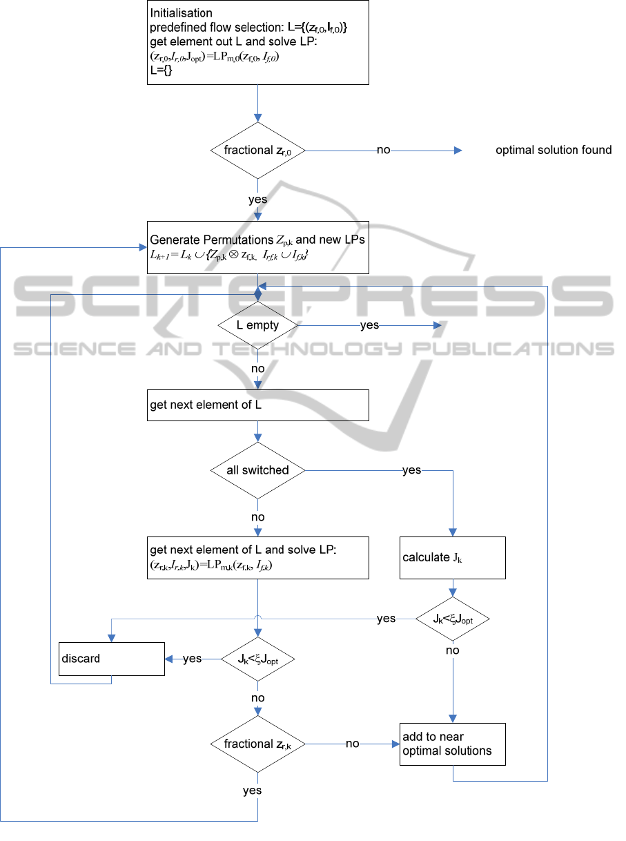
Figure 3: Schematic flow diagram for the mixed-integer search procedure.

ICINCO2013-10thInternationalConferenceonInformaticsinControl,AutomationandRobotics

502

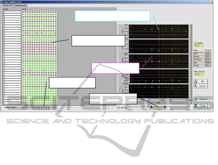
Figure 4: Graphic interface for integer solutions in the vicinity of the anchor continuous solution.

solution domain in order to specify an anchor, for a

particular selected final product stream. This search

is guided by well-structured graphic overviews and

flexible input possibilities as shown in the previous

work (Keller and Agarwal, 2012). After a

continuous-solution anchor has been selected for the

final product stream, the user clicks a button to

switch to the integer-solution mode, which

calculates and displays the mixed-integer solutions

in the vicinity of the anchor continuous solution,

using the solution procedure described above.

The user interface for displaying these results is

shown in Fig. 4. Since slightly sub-optimal solutions

might get prefered by the user based on

considerations not available in the above problem

formulation, and since several near-optimal

solutions might yield objective-function values quite

close to each other, the tool displays all such results

in a convenient overview, and allows the user to

flexibly and comfortably select the particular

solution that is best in view of the other

considerations.

On the left-hand side of the graphic interface in

Fig. 4, the user sees, for the particular final product

stream at hand, which intermediate product streams

would be used (value 1, colour green, shade light

gray) and which would not be used (value 0, colour

red, shade dark gray). Each relevant solution is

thereby shown in a single column. At the bottom of

this part of the display, the user can provisionally

select one particular solution by clicking it green (or

shade light gray).

On the right-hand side of the graphic interface,

the user sees, for the various solutions, the values of

the physical properties versus the yield of the final

product stream at hand. Thereby, the solution

selected on the left-hand side, as well as the anchor

solution (as intersecting dash-dotted lines), are

highlighted for easier judgment. At the bottom of

this part of the display, the user can select a range of

yields in order to narrow down the number of

solutions that are displayed on the left-hand side.

5 RESULT

Tests in industrial cases confirmed that the tool

fulfils the requirements of ease-of-use and

flexibility. The results shown in the overview

graphics were judged by the users as extremely

useful. A decisive factor for the positive judgment

by the users and their eagerness to use the tool was

the relative quick reaction time of the computation

 in the range of 10 – 20 seconds, whenever the

user klicks the button for computing discrete

solutions around the continuous-solution anchor,

and

 without any perceptible delay, whenever the user

changes any other input.

Compared to the manual decision making, the

tool-supported decision showed a value increase of

Selected solution

Selection of streams

Physical property for chosen solution

Selected yield range

Spli

-mode solution

PerformanceOptimizationinIntelligentManufacturing-DecisionSupportSystemforValueEngineeringinFlourMills

503

about 5%, which is considerable in this industry.

6 CONCLUSIONS

A novel decision-support tool is presented that

solves the problem of optimally allocating each of

many intermediate product streams in flour mills to

one of a few final product streams, while accounting

for uncorrelated physical properties of the streams,

a-priori unknown properties and yields of the final

product streams, and the lack of explicit formulation

of "value" of the final product streams with respect

to their physical properties. A fast solution strategy

is developed that decouples the original problem into

simpler problems for each final product stream, uses

a fictitious continuous-space solution as an initial

facilitating anchor, and computes several integer

solutions in the vicinity of the anchor by combining

Branch-and-Bound with multiple Linear

Programming steps complemented by a relaxation

scheme. The developed optimization solution

enables display of results without annoying time lag,

whenever the user changes any input in the user-

interface.

In many mills, the relevant physical properties of

the intermediate and the final product streams may

include properties that do not “mix” linearly. The

linearity with respect to the physical properties is a

fundamental assumption in the above solution

procedure, so that the tool cannot be used in cases

where one or more properties “mix” nonlinearly.

Fundamentally different solution procedures have

been devised and implemented for this situation, and

are currently being tested and refined.

REFERENCES

Borghetti, A., Paolone, M., Nucci, C. A., 2011. A Mixed

Integer Linear Programming Approach to the Optimal

Configuration of Electrical Distribution Networks with

Embedded Generators, 17th Power Systems

Computation Conference, Stockholm, Sweden.

Chen, D.-S., Batson, R. G., Dang, Y., 2010. Applied

Integer Programming: Modeling and Simulation, John

Wiley & Sons, Inc., New York, NY.

Guan, X., Zhai, Q., Papalexopoulos, A., 2003.

Optimization Based Methods for Unit Commitment:

Lagrangian Relaxation versus General Mixed Integer

Programming, IEEE Power Engineering Society

General Meeting, 2(4), 2666.

Hansen, P., Jaumard, B., Savard, G., 1992. New Branch-

and-Bound Rules for Linear Bilevel Programming,

SIAM J. Sci. and Stat. Comput., 13(5), 1194-1217.

Keller, J. P., Agarwal, M., 2012. Fast, Flexible, Interactive

Decision-Support Tool: An Industrial Application, 8th

International Symposium on Intelligent and

Manufacturing Systems, Adrasan, Turkey.

Lawler, E. L., Wood, D. E., 1966. Branch-and-Bound

Methods: A Survey, Operations Research, 14(4), 699-

719.

Lee, M. L., Kim, J.-G., Kim, Y.-D., 2009. Linear

Programming and Lagrangian Relaxation Heuristics

for Designing a Material Flow Network on a Block

Layout, International Journal of Production Research,

47(18), 5185-5202.

Leyffer S., 2001. Integrating SQP and Branch-and-Bound

for Mixed Integer Nonlinear Programming,

Computational Optimization and Applications, 18,

295-309.

Vielma J. P., Ahmed S., Nemhauser G. L., 2008. A Lifted

Linear Programming Branch-and-Bound Algorithm

for Mixed Integer Conic Quadratic Programs,

INFORMS Journal on Computing, 20, 438-450.

Wolsey, L. A., 1980. Heuristic Analysis, Linear

Programming and Branch and Bound, Mathematical

Programming Studies, 13, 121-134.

ICINCO2013-10thInternationalConferenceonInformaticsinControl,AutomationandRobotics

504