A Bayesian Approach to FDD Combining Two Different Bayesian
Networks Modeling a Data-Driven Method and a Model-based Method
Mohamed Amine Atoui, Sylvain Verron and Abdessamad Kobi
LASQUO/ISTIA, L’UNAM University, 62 Avenue Notre Dame du Lac, 4900, Angers, France
Keywords:
FDD, Data-Driven Methods, Model-based Methods, Incidence Matrix, Bayesian Networks, Water Heater
System.
Abstract:
In this paper, we present an original FDD method. The interest of this method is her ability to coexist residuals
and measures, under a same and a single tool. Indeed, our proposal is to combine two different Bayesian
networks to FDD. A model-based method is associated to a data-driven method to enhance decision making
on the system operating state. This method is evaluated on a simulation of a water heater system in some
various circumstances.
1 INTRODUCTION
Nowadays, monitoring methods (also known as Fault
Detection and Diagnosis methods (FDD)) are more
and more used, due to the increasing systems com-
plexity. They contributeto the reduction of faults or in
the ideal case for their elimination by an entity (oper-
ator, engineer, automaton...) which will examine the
state of malfunction caused by these past and makes
a decision about the future of the system (adjusting
settings, maintenance, closure...). These methods are
used to describe and explain, at each instant, the situ-
ation in which the system is situated. They consist of
two phases usually associated: detection and diagno-
sis phases.
The detection phase seeks to confirm if the sys-
tem is still in normal operating state (In control) or is
not (Out of control). The diagnosis phase is used in
order to designate the faults responsible for the devia-
tion of the system of his normal operating. This phase
can be defined in different ways depending on the de-
sired description level. According to (Chiang et al.,
2001) we can distinguish three definitions: identifica-
tion (determine the susceptible measures explaining
the occurred fault on the system), isolation (distin-
guishes the measure responsible for system abnormal
functioning), diagnosis (explains the faults occurred
in the system by expressing their type, location, am-
plitude and duration).
In the last years, many monitoring methods have
emerged (Chiang et al., 2001; Isermann, 2006; Qin,
2006; Ding, 2008). Among them, we can distin-
guish two classes of methods: model-based meth-
ods and data-driven methods. Model-based meth-
ods use a priori knowledge of the system for ex-
plaining its dynamic behavior. This knowledge cor-
responds to a specific set of mathematical equations
representing the dependencies that exist between the
variables of the system and contributing to the gener-
ation of residuals (differences between observed and
estimated measurements when the system is supposed
in normal operation). Once generated, their evalua-
tion contributes to the understanding of the operating
state. In contrast, data-driven methods are based only
on measures taken at different times, and analyzed in
relation to a historical of data regarding the system.
The ability of the data-driven methods to manage
a significant number of data associated with the ca-
pacity of the model-based methods to describe ac-
curately the dynamic behavior of the system and
to provide a physical understanding, might improve
the monitoring, increase the number of scenarios
taken into account, benefit from the advantages of
both methods and to struggle against the individual
shortcomings of each one when they are used sepa-
rately. However, despite many researchers (Chiang
et al., 2001; Venkatasubramanian et al., 2003; Ding
et al., 2009) suggesting that the creation of a common
framework using both classes of methods, would al-
low a better monitoring system, these research fields
remain unexplored. Nevertheless, we can find some
recent works in the literature describing different as-
sociation of the two methods.
In (Schubert et al., 2011) a unified scheme is pro-
162
Amine Atoui M., Verron S. and Kobi A..
A Bayesian Approach to FDD Combining Two Different Bayesian Networks Modeling a Data-Driven Method and a Model-based Method.
DOI: 10.5220/0004432101620168
In Proceedings of the 10th International Conference on Informatics in Control, Automation and Robotics (ICINCO-2013), pages 162-168
ISBN: 978-989-8565-71-6
Copyright
c
 2013 SCITEPRESS (Science and Technology Publications, Lda.)

posed. The authors combine subspace approachesand
univariate and multivariate statistical control meth-
ods (data-driven methods) with inputs reconstruc-
tion method and banks of Unknown Input Observer
(model-based methods). Luo et al. (Luo et al., 2010)
for antilock braking system (ABS), propose a hybrid
approach using parity equations and a nonlinear ob-
server for residuals generation. These residuals are
used by statistical tests with the aid of SVM (sup-
port vector machine) to detect and isolate different
faults that may occur in the system. In (Ghosh et al.,
2011), for monitor a laboratory distillation column a
fusion of decisions of several monitoring methods is
proposed. The authors use four monitoring methods:
a model-based method: an extended Kalman filter,
and three data-driven methods: SOM (Self Organized
Map), artificial neural network and PCA (Principal
Component Analysis). The output of each method
corresponds to an assignment to one class of fault. A
fusion strategy is then applied using them to make the
right decision (Bayesian decision and other). Yew et
al. (Yew and Rajagopalan, 2010) propose collabora-
tion between different methods under a multi-agent
framework using some decision fusion methods.
The proposals mentioned above, although inter-
esting for the combination of data-driven and model-
based methods, does not seem to cover or address a
particular problem which is the lack of information
or approximations of the system (decrease in perfor-
mance of monitoring). We believe that the combina-
tion of the two methods is mainly interesting when the
two methods are able to complete their information
and to finally provide better oversight. For example,
a combination of a model-based method, without an
accurate model, and a data-driven method, with some
data are missing or insufficiently represented. In this
paper, we propose a new monitoring method based
on Bayesian networks. This method uses the comple-
mentarities that may have a data-driven and a model-
based method in a single and common tool. The ma-
jor interest of this combination is their ability to im-
prove the decision making when the two methods suf-
fer from a information lack or an approximations of
the system (decrease in performance of monitoring).
The paper is structured as follows: in section 2
we introduce Bayesian networks followed by a short
description of data-driven and model-based methods
in sections 4 and 3; section 5 describes the monitor-
ing methodology proposed; finally, the results of the
proposed method obtained in different conditions on
a simulation of a water heater system are outlined in
the last section.
2 BAYESIAN NETWORKS
A Bayesian network (Buntine, 1996; Jensen, 1996),
is a probabilistic directed acyclic graph. Each node in
the network represents a random variable that may be
discrete with n modalitees (multinomial) or continue
(univariate or multivariate). Each node has a condi-
tional probability table (marginal probability table for
root nodes). The oriented arcs show the conditional
dependencies/independencies that exist between dif-
ferent nodes of the graph. Each directed arc can link
only two nodes: among these nodes, one is called the
father and the other, the son. For updating the network
and calculate the different a posteriori probabilities
corresponding to each node, given the availability of
new information on the network (evidence), calcula-
tions (eg: Bayes rule) named inference is required. A
Bayesian network, in general, can be defined formally
by:
• a directed acyclic graph G, G=(V,E), where V the
set of nodes of G, and E the set of arcs of G,
• E is a finite probabilistic space (Ω,Z, p), with Ω a
non-empty space, Z a set of subspace of Ω and p
a probability measure on Z with p(Ω) = 1,
• a set of random variables associated with to the
nodes of the graph G and defined on (Ω,Z, p),
such that:
P(V
1
,V
2
,...,V
n
) =
n
∏
i=1
p(V
i
|C(V
i
)) (1)
where C(V
i
) is the set of parent nodes of V
i
in the
graph G.
Nowadays, several variants of Bayesian networks
exist. One of them is the Bayesian network calssifier,
who is based on a discrete root node modelling the
fact of belonging to one class among others. Note that
under the assumption of dependence/independence of
variables X emitted, several types of structures are
proposed (Friedman et al., 1997). Among them, we
use two kind of Bayesian networks classifiers: one is
the Naive Bayes network, it’s making the strong as-
sumption that the variables are class conditionally in-
dependent and the second network is the semi-naive
condensed Bayesian network who provides a simple
structure that take into account correlation that may
exist under a group of variables.
3 BAYESIAN NETWORK AND
MODEL-BASED METHODS
The model-based methods, in the presence of an
analytical representation of the system, use resid-
ABayesianApproachtoFDDCombiningTwoDifferentBayesianNetworksModelingaData-DrivenMethodanda
Model-basedMethod
163

uals generators (Isermann, 2006) which as their
name suggests, contribute to the creation of residu-
als (r
1
,··· ,r
n
)
T
(the difference between the existing
measures on the system and their estimates). Once
generated a consistency test (evaluation of residuals)
is triggered to check if no residual is different from
zero. Indeed, during normal operating, the residu-
als are assumed to be equal to zero. However, some-
times they are not only sensitive to the faults but also
the noise measurements performed on the system, to
the disturbances and the modeling errors, makes them
different to zero even during normal operation, that’s
why generally each residual is considered to be sta-
tistically null with a given variation (eg: a residual
follows a normal distribution, with a standard mean
µ = 0 and variance σ
2
= 1). Thus, generally binary
statistical tests are used to making decision between
H
0
(corresponding to the distribution of residuals dur-
ing normal operating) and H
1
the alternative hypoth-
esis (corresponding to faults). This is achieved by at-
tempting to minimize the risk of first and second kind,
respectively, α and β (see Figure 1).
Figure 1: Statistical test.
The result of residuals evaluation (u
t
1
,..., u
t
n
)
T
, in
the case of the diagnostic methods based on structured
residuals (constructed in order to be sensitive to cer-
tain faults and not to others), is compared (usually
a logic test) to another vector representing the char-
acteristics of each fault F
j
∈ {F
1
,F
2
,..., F
k
}. These
characteristics are generally assembled into a binary
array called incidence matrix (an example is shown in
Figure 1).
Table 1: Example of incidence matrix.
IC F
1
F
2
... F
k
u
1
0 b
1.2
b
1.3
... b
1.k
u
2
0 b
n.2
b
2.3
... b
2.k
.
.
.
.
.
.
.
.
.
.
.
.
.
.
.
.
.
.
u
n
0 b
n.2
b
n.3
... b
n.k
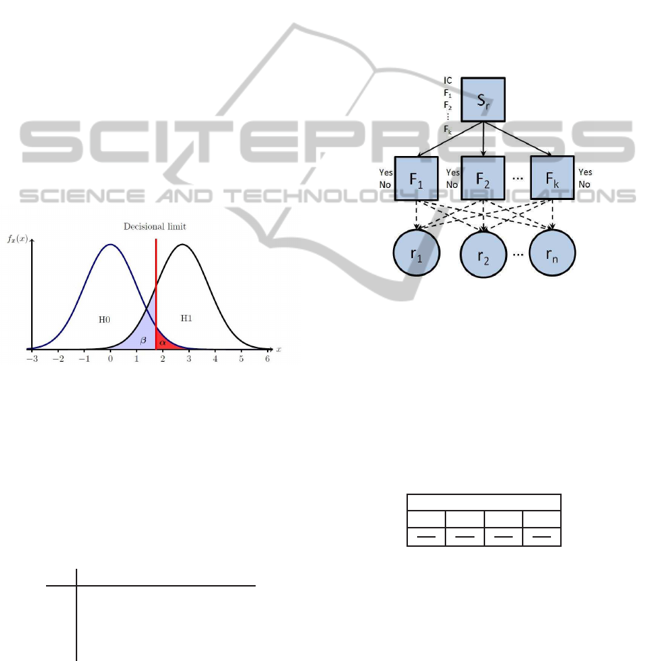
Furthermore, in (Verron et al., 2009), Verron
et al. model the last two phases of the model-
based monitoring (knowing that monitoring methods
based model usually consists of three complemen-
tary phases: generation of residuals, residual evalu-
ation (change detection) and decision making (diag-
nosis)). They propose a combination of two Bayesian
networks works (modeling a control chart T
2
(Verron
et al., 2007) and the modeling of the incidence ma-
trix (Weber et al., 2008)). To achieve this, a hybrid
Bayesian network, representing k naive Bayesian net-
work, is proposed. This network is made of discrete
nodes (representing the k faults) with two modalities
({presence (yes) and not presence (No) of F
j
}) and
continuous nodes (representing the n residuals) con-
sidered as a standard Gaussian variable (with a mean
µ and variance σ
2
).
Figure 2: Bayesian network for model-based monitoring.
In order to combine explicitly the probabilities of
belonging to one of the three faults (corresponding to
the states of the system when it is out of control) and
the probability that the system is always in normal
operating state IC, we propose to add to the network
a discrete parent node S
r
with k+1 modalitees (see 2)
linked to all the other nodes F
j
.
The conditional probability tables (CPT) of the
node S
r
and his son nodes F
j∈1,...,k
are given in tables
2 and 3.
Table 2: CPT of the node S
r
.
S
r
IC F
1
... F
k
1
k+1
1
k+1
1
k+1
1
k+1
4 BAYESIAN NETWORK AND
DATA-DRIVEN METHODS
Unlike methods that require an accurate model de-
signed from first principles as a priori knowledge
of the system, this methods try to detect and ex-
plain a change in the normal operating system, rely-
ing solely on measurements collected on the system
ICINCO2013-10thInternationalConferenceonInformaticsinControl,AutomationandRobotics
164

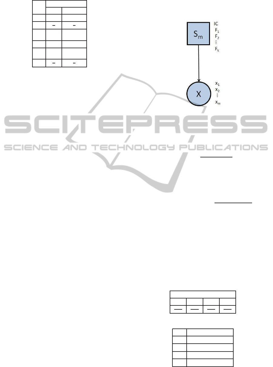
Table 3: CPT of the nodes F
1
&F
2
&. ..F
k
.
S
r
F
1
&F
2
&...F
k
Yes No
IC 0 1
F
1
1
2
1
2
.
.
.
.
.
.
.
.
.
F
k
1 0
.
.
.
.
.
.
.
.
.
F
n
1
2
1
2
(temporary or not). Several data-driven methods for
monitoring purpose exist, they depends on the avail-
ability or unavailability of historical data on the sys-
tem. Among this methods, we can firstly mention the
subspace methods SMI (Subspace Model Identifica-
tion)(Overschee and Moor, 1996), a linear identifica-
tion algorithms, developed to address the problems of
building an accurate model for complex systems. The
principal component analysis (ACP) (Harkat et al.,
2006), is a statistical method that can be used to
modelise existing dependences between a set of sys-
tem variables or as a method of data reduction (used
when the number of variables is considerable). Men-
tion may also the control charts methods (MacGregor
and Kourti, 1995), statistics gathered over a period of
time t, which are also widely used in industry. They
(control chart T
2
of Hotelling, MEWMA (Multivari-
ate Exponentially Weighted Moving Average) are de-
signed to monitor the normal operation of the system.
Otherwise, when a history of faults is available,
supervised classification methods, adapted to the di-
agnostic can be used. Indeed, the diagnosis prob-
lem can be formulated for a given observation, as
a problem of discrimination between several operat-
ing modes. Among this data-driven methods, we can
mention neural networks (Duda et al., 2001), SVM
(support vector machine) (Steinwart and Christmann,
2008), discriminant analysis (Fukunaga, 1990) (can
be modelled under a Bayesian network, where the
variables are assumed follow a multivariate normal
distribution).
In our work, one assuming our knowledge about
the faults covers almost all the space (assumed as
closed space) out of control (H
1
⊆ {F1,... , F
k
}), we
propose to use a Bayesian network classifier to dis-
criminate between these faults and the state IC (where
the system is considered in normal operating condi-
tion H
0
). To achieve this, we use a Bayesian Network
(see figure 3) naive semi condensed (RBNSC) con-
sisting of a discrete node representing k+1 modalities
and continuous multivariate Gaussian node (with a
mean µ and variance Σ estimated on the fault database
by Maximum Likelihood Estimation (MLE) (Duda
et al., 2001)) combining all the m variables of the sys-
tem (x
1
,x
2
,..., x
m
).
Figure 3: Bayesian network for data-driven monitoring.
By making assumption about normality of each
modality, this network using a decision rule based on
the Bayes formula (2):
P(Y/X) =
P(Y)P(X/Y)
P(X)
(2)
corresponds to a quadratic discriminant analysis (5) :
δ : x ∈ M
∗
j
, if j
∗
= argmax
j=1,...,k+1
{P(M
j
/x)} (3)
= argmax
j=1,...,k+1
{
P(M
j
)P(x/M
j
)
P(x)
} (4)
= argmax
j=1,...,k+1
{P(M
j
)P(x/M
j
)} (5)
Where P(M
j
/x) is the probability a posteriori of
Y, P(x) is the density function of x, P(x/M
j
) is the
likelihood and P(M
j
) the prior probability of M
j
Thus, it making us able to decide to a given
instant, in which operating state, the system be-
longs among its various states separated quadratically
(IC, F
1
,F
2
,..., F
k
). The probability tables for each
node are shown in the tables 4, 5.
Table 4: CPT of the node S
m
.
S
m
IC F
1
... F
k
1
k+1
1
k+1
1
k+1
1
k+1
Table 5: CPT of the node X.
S
m
X
IC X ∼ N(µ
IC
,σ
2
IC
)
F
1
X ∼ N(µ
F
1
,σ
2
F
1
)
... ...
F
k
X ∼ N(µ
F
k
,σ
2
F
k
)
ABayesianApproachtoFDDCombiningTwoDifferentBayesianNetworksModelingaData-DrivenMethodanda
Model-basedMethod
165

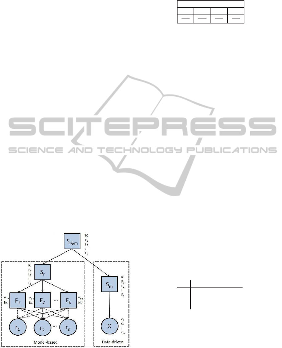
5 DECISION FUSION
To improvethe decision making, in this work, we pro-
pose to combine the two monitoring methodology in a
same and a single tool. Indeed, our proposal consists
to combine the two methods discussed above under a
Bayesian network.
Thus to build our new network combining both
methods, a new discreet node S
r&m
is added (see fig-
ure 4). This node represents like the root nodes S
r
and S
m
a variable with j + 1 modalities. One of these
corresponds to normal operating condition (IC) where
the other modalities j corresponds to the known faults
that may occur on the system. This new node S
r&m
is used to connect the two root nodes and so asso-
ciate the both methods by fusioning their decisions.
Thus, a conjunctivecombination (see (Xu et al., 1992;
Chen et al., 1997) for others decision fusion methods)
is made under the assumption that the two network
are conditionally independent to the node added. In-
deed, thanks to the use of the Bayes formula (2), the
Bayesian network offers a naturally probabilistic fu-
sion capacity.
Once the network is built, we enter the observa-
tions (evidences) in the network. They correspond to
the residuals obtained and the measures taken on the
system at a given instant. These evidences are then
transmitted to other unobserved nodes in the network.
Their marginal probabilities are then calculated us-
ing the inference method employed (we use junction
tree). After having carried out this inference, the node
S
r&m
indicates for each k+ 1 modalities, the probabil-
ity of its occurrence.
Figure 4: A two combination methods.
Regarding the decision, among others criterions,
we chose to use the maximum a posteriori like we
do for the others methods (model-based, data-driven),
Table 6: CPT of the node S
r&m
.
S
r&m
IC F
1
... F
k
1
k+1
1
k+1
1
k+1
1
k+1
where the modality with the higher probability a pos-
teriori is choose. The table of conditional probabili-
ties of node S
r&m
is shown in table 6.
6 APPLICATION
To illustrate our approach, we use a simulation of a
water heater. It consists of a tank equipped with two
resistors R
1
and R
2
. The inputs are the water flow rate
Q
i
, the water temperature T
i
and the electric power for
heating P. The outputs are the rate of water flow Q
0
and the temperature T regulated around an operating
point. The temperature of the incoming water T
i
is
assumed constant.
The objective of the system is to provide a water
flow at a given temperature. Using hydraulic and ther-
mal equations, in this analysis, only sensor faults are
considered: water level sensor H, temperature sensor
T, sensor flow of water from Q
0
. The detailed math-
ematical model of the system is presented in (Weber
et al., 2008).
A classic residuals generator is used: a Luen-
berger observer. The output vector is [H,T]
T
and
the input vector [Q
i
,P]. Structured residuals [r
1
,r
2
,r
3
]
are generated and evaluated to detect faults of water
level sensor H and temperature sensor T. Accord-
ing to the physical equations between the flow rate
Q
0
and the liquid level H, other residual can be estab-
lished. The incidence matrix (the link between symp-
toms [u
1
,u
2
,u
3
] and faults [T,H,Q
0
]) defined in table
7 will give the structure of our Bayesian network.
Table 7: Incidence Matrix of the heating water system.
IC T H Q
0
u
1
0 1 0 0
u
2
0 0 1 0
u
3
0 0 1 1
We simulated the system according to the sce-
narios described in table 8 in order to test the pro-
posed method under different assumptions. Indeed,
the value of combining the two methods is to be able
to benefit of good results even when one or the other
method is not very efficient (missing detection of ab-
normal operating state, faults misdiagnosis). Thus,
we propose to test the Bayesian network, taking into
account an accurate model (M+) or a less accurate
ICINCO2013-10thInternationalConferenceonInformaticsinControl,AutomationandRobotics
166

(M−), and a complete dataset of suitable size (D+)
or incomplete dataset (a lack faults data, a few data)
(D−). Thus, the scenarios previously presented will
be tested on four assumptions described in 9.
Table 8: Simulated scenarios.
period 1-30 31-60 61-90 91-120
case In Control faultT faultH faultQ
0
Table 9: Hypothesis matrix.
hypothesis M(Model) D(Data)
H
I
M
+
D
+
H
II
M
+
D
−
H
III
M
−
D
+
H
VI
M
−
D
−
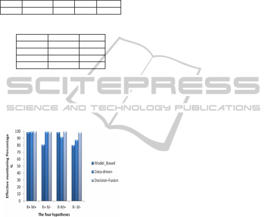
Every simulation was performed using Mat-
lab/Simulink and BNT (BayesNet Toolbox). For each
observation, we attribute the fault to the modality with
the greater a posteriori probability. The different re-
sults of the simulation obtained by testing our meth-
ods under four different assumptions are presented in
figure 5.
Figure 5: Simulations results under the four hypothesis.
One can notice that for each hypothesis, the pro-
posed method can usually equalize the performance
of each method and even to improve the monitoring.
In hypothesis I, the three methods are good, they give
right answers. The proposed method is slightly more
efficient. For the hypothesis II, we suppose that the
data of the fault H misses us. In this condition, we see
that the method proposed can have good results. The
same thing is happen, in the case of the third hypothe-
sis, where we have degraded the model. Finally, in the
hypothesis VI, the proposed approach allows a better
decision than the two other methods. This shows that
the proposition made is efficient and can take advan-
tage of the two basic methods under a Bayesian net-
work.
7 CONCLUSIONS
The interest of this paper is to present a new method
for monitoring industrial systems. We have presented
a particular structure of Bayesian network which con-
sists of discrete and Gaussian nodes allowing to mod-
els and combines two Bayesian networks dedicated
to monitoring: one for data-driven monitoring and
one representing the incidence matrix and the eval-
uation of residuals for the model-based monitoring.
This original structure can enhance decision mak-
ing during monitoring using simultaneously data and
residuals. This method has been tested on a water
heater system, where an improvement of the decision
is made and this in the most cases (specific model,
model degraded and more or less data).
REFERENCES
Buntine, W. (1996). A guide to the literature on learning
probabilistic networks from data.
Chen, K., Wang, L., and Chi, H. (1997). Methods of com-
bining multiple classifiers with different features and
their applications to text-independent speaker identifi-
cation. International Journal of Pattern Recognition
and Artificial Intelligence, 11:417–445.
Chiang, L., Russel, E., and Braatz., R. (2001). Fault Detec-
tion and Diagnosis in Industrial Systems. Springer.
Ding, S. (2008). Model-Based Fault diagnosis Techniques.
Springer-Verlag, Berlin.
Ding, S., Zhang, P., Naik, A., Ding, E., and Huang, B.
(2009). Subspace method aided data-driven design of
fault detection and isolation systems. Journal of Pro-
cess Control, 19(9):1496 – 1510.
Duda, R. O., Hart, P. E., and Stork, D. G. (2001). pattern
classification 2nd edition. Wiley.
Friedman, N., Geiger, D., and Goldszmidt, M. (1997).
Bayesian network classifiers. Machine Learning,
29:131–163.
Fukunaga, K. (1990). Introduction to statistical pattern
recognition (2nd ed.). Academic Press Professional,
Inc., San Diego, CA, USA.
Ghosh, K., Ng, Y. S., and Srinivasan, R. (2011). Evaluation
of decision fusion strategies for effective collaboration
among heterogeneous fault diagnostic methods. Com-
puters & Chemical Engineering, 35(2):342 – 355.
Harkat, M.-F., Mourot, G., and Ragot, J. (2006). An im-
proved pca scheme for sensor fdi: Application to an
air quality monitoring network. Journal of Process
Control, 16(6):625 – 634.
Isermann, R. (2006). fault-diagnosis system. Springer, in
robotics (vol. xviii) edition.
Jensen, F. (1996). An Introduction to Bayesian Networks.
Taylor and Francis, London, United Kingdom, Lon-
don, United Kingdom.
ABayesianApproachtoFDDCombiningTwoDifferentBayesianNetworksModelingaData-DrivenMethodanda
Model-basedMethod
167

Luo, J., Namburu, S. M., Pattipati, K. R., Qiao, L., and
Chigusa, S. (2010). Integrated model-based and data-
driven diagnosis of automotive antilock braking sys-
tems. IEEE Transactions on Systems, Man, and Cy-
bernetics, Part A, 40(2):321–336.
MacGregor, J. and Kourti, T. (1995). Statistical process
control of multivariate processes. Control Engineer-
ing Practice, 3(3):403 – 414.
Overschee, P. V. and Moor, B. D. (1996). Subspace Identi-
fication for linear systems: Theory - Implementation -
Applications. Kluwer Academic Publishers.
Qin, S. J. (2006). An overview of subspace identifica-
tion. Computers and Chemical Engineering, 30:1502
– 1513.
Schubert, U., Kruger, U., Arellano-Garcia, H., de Sa Feital,
T., and Wozny, G. (2011). Unified model-based fault
diagnosis for three industrial application studies. Con-
trol Engineering Practice, 19(5):479 – 490.
Steinwart, I. and Christmann, A. (2008). Support Vector
Machines. Springer Publishing Company, Incorpo-
rated, 1st edition.
Venkatasubramanian, V., Rengaswamy, R., Kavuri, S. N.,
and Yin, K. (2003). A review of process fault de-
tection and diagnosis: Part iii: Process history based
methods. Computers & Chemical Engineering,
27(3):327 – 346.
Verron, S., Tiplica, T., and Kobi, A. (2007). Multivariate
control charts with a bayesian network. In 4th Interna-
tional Conference on Informatics in Control, Automa-
tion and Robotics (ICINCO’07), pages 228–233.
Verron, S., Weber, P., Theilliol, D., Tiplica, T., Kobi, A., and
Aubrun, C. (2009). Decision with bayesian network in
the concurrent faults event. In 7th IFAC Symposium on
Fault Detection, Supervision and Safety of Technical
Processes (SafeProcess’09).
Weber, P., Theilliol, D., and Aubrun, C. (2008). Component
Reliability in Fault Diagnosis Decision-Making based
on Dynamic Bayesian Networks. Proceedings of the
Institution of Mechanical Engineers Part O Journal of
Risk and Reliability, 222(2):161–172.
Xu, L., Krzyzak, A., and Suen, C. Y. (1992). Methods of
combining multiple classifiers and their applications
to handwriting recognition. IEEE Transactions on
Systems, Man, and Cybernetics, 22(3):418–435.
Yew, S. N. and Rajagopalan, S. (2010). Multi-agent
based collaborative fault detection and identification
in chemical processes. Engineering Applications of
Artificial Intelligence, 23(6):934 – 949.
ICINCO2013-10thInternationalConferenceonInformaticsinControl,AutomationandRobotics
168