
Enhancing the Life Time of a Wireless Sensor Network in Target
Tracking Applications
Phuong Pham and Sesh Commuri
School of Electrical and Computer Engineering, The University of Oklahoma, Norman, Oklahohoma, U.S.A.
Keywords: Wireless Sensor Networks, Target Tracking, Energy Efficiency, Kalman Filters.
Abstract: We propose a method to enhance the life span of the WSN under the constraint of tracking quality. The
problem is cast as an optimization problem to minimize the power consumption cost function under the
constraint of tracking quality. The cost function accounts for both the residual power of each sensor node and
its sensing task. The cost function increases when the residual power of a sensor node decreases or a sensing
task requires more power. The improvement in the tracking performance obtained by the proposed method is
demonstrated through numerical examples.
1 INTRODUCTION
Target tracking is one of the important applications
of a Wireless Sensor Network (WSN). Difficulties in
the deployment of WSNs and the limited capabilities
of each node restrict their long term utility for most
applications. Some of the challenges that need to be
addressed are the energy consumption, useful life,
and quality of information obtained using these
networks. These problems take on added importance
in target tracking applications where the target is
mobile and the sensor measurements are noisy.
Energy consumption and tracking quality
(Demigha et al., 2012), (Zhao et al., 2002) are two
main challenges in tracking of a dynamic target using
WSNs. To save energy consumption, Fang and Li
(Fang and Li, 2009) proposed a distributed
estimation method for reducing communication and
compressing data. Other approach (Cui et al., 2007)
minimized quantization error and transmission
power. Lin et al., 2009 investigated the energy-
efficient multiple sensor scheduling, and calculated
the optimal sampling time to meet the tracking
performance. Several sensor activation schemes were
used in (Pattem et al., 2003) to reduce power
consumption under the effect of tracking quality.
Information content-based sensor selection algorithm
was proposed by (Onel et al., 2009). The
optimization approaches (Masazade et al., 2012),
(Mukherjee et al., 2011) were proposed to reduce
overall power consumption of sensor networks.
Smart scheduling methods (Atia et al., 2011),
(Fuemmeler et al., 2011) were proposed to activate
appropriate sensors for the tracking and to deactivate
the “low-quality” sensors. The main purpose of
these methods is to save the energy consumption and
to prolong the network life time. Moreover, the
tracking quality metrics, defined in these works, did
not address the relationship between trilateration
uncertainty and geometric distribution of sensor
nodes.
To track a dynamic target using range-
measurement sensors, the trilateration uncertainty is
used as a main metric for tracking quality
(Manolakis, 1996), (Yang and Liu, 2008), (Powers,
1966), (Thomas and Ros, 2005), (Fang, 1986), which
depends on both the sensors’ locations and the
location of the target. Thus, a small number of sensor
nodes can result in small tracking errors while a large
number of nodes may result in poor tracking
performance.
In this paper, we proposed a method to improve
the life span of the WSN while maintaining the
desired level of tracking quality. The problem is
formulated as an optimization problem which
minimizes the power consumption under the
constraint of tracking quality. The power
consumption cost depends on two parameters: the
current residual power and the power expected to be
consumed for a sensing mode. The cost is inversely
proportional to the residual power of the node. Each
sensor node operates in four modes (sleeping, active,
sensing, and master mode) sorted as increasing
373
Pham P. and Commuri S..
Enhancing the Life Time of a Wireless Sensor Network in Target Tracking Applications.
DOI: 10.5220/0004432503730379
In Proceedings of the 10th International Conference on Informatics in Control, Automation and Robotics (ICINCO-2013), pages 373-379
ISBN: 978-989-8565-70-9
Copyright
c
2013 SCITEPRESS (Science and Technology Publications, Lda.)

power consumption; a sleeping node consumes much
less power than a master node does. By minimizing
the power consumption cost under the constraint of
trilateration uncertainty, the nodes with more residual
power are scheduled for more power-intensive tasks,
while the nodes with low battery power are
scheduled to be in sleeping mode. The selection
algorithm is suboptimal while the computational cost
is significantly reduced. Moreover, the algorithm is
implemented in a distributed manner, and is scalable
to a network of a larger number of sensor nodes. The
Kalman filter is proposed to further improve tracking
quality. At a time instant, only one master node plays
a role as the fusion center, which runs the Kalman
filter and the selection algorithm. The mathematical
analysis and numerical simulations will verify the
effectiveness of the tracking algorithm.
2 PROBLEM FORMULATION
We consider the problem of target tracking using a
wireless sensor network. A two-dimensional sensor
field is densely deployed with stationary sensor
nodes, which are equipped with transceivers,
computational platforms, and range measurement
units. When a target presents in the sensing field, the
challenge is to schedule sensor operating modes
(sleeping, active, sensing, or master mode) (1) to
increase network life time and (2) to the required
tracking quality. The proposed power consumption
cost for using a specific sensor is a deceasing
function with respect to its residual power. The
optimization problem selects a set of sensor nodes
that minimizes the power cost function under the
constraint of trilateration uncertainty. The sensor
selection algorithm also enables the distributed
implementation of the tracking algorithm, i.e.,
Kalman filter.
2.1 Power Consumption Model
and Cost Function
The power consumption cost function accounts for
two conditions: the residual power of each node and
its operating modes. To simplify the problems, it is
assumed that each node has four operating modes
(sorted as increasing power consumption) including:
sleeping mode, active mode, sensing mode, and
master mode. Moreover, the power consumption of
each sensor in a particular operating mode is
constant.
Let be the total number of sensor nodes in the
sensor field. Let
,
,…
, where
represents the operating mode of the
node, and
∈
0,1,2,3
(the values 0,1,2 and 3 represent
sleeping, active, sensing, and master mode,
respectively).
Let the normalized residual power of a node be
(if0, the node is depleted, while 1 the node
has its full power). Let :0,1↦0,∞ be a
continuous and decreasing function. Let
and
be
normalized residual power and normalized power
consumption, respectively, in one tracking interval.
The power consumption cost for the
node is
defined as
.
(1)
The total cost function of the network in one tracking
interval is given as
∑
.
2.2 Rilateration Algorithm
The measurement model is given by the following
equation
‖
‖
,
(2)
where
‖
.
‖
is standard Euclidean norm;
∈
is
the position of
sensor;
∈
is the position of
the target;
∈ is the distance measurement; and
~0,
is the noise measurement.
Suppose that
sensors can sense the target,
resulting in
nonlinear measurement equations (2).
For each pair of integers
,
, 1
, the
and
in (2) are squared and subtracted to
represent the measurement in the linear form. The
location of the target
, the least square
trilateration algorithm, is given by
.
(3)
where
∈
,
, and
∈
.
…
and
…
.
2
,
‖
‖
where ,. The map :1
1
↦1 is one-to-one.
The tracking system is given by the following
two equations.
.
(4)
.
(5)
ICINCO2013-10thInternationalConferenceonInformaticsinControl,AutomationandRobotics
374

Where
∈
is the state of the target (location
and velocity),
~0,
: the process noise with
covariance matrix
.
∈
is location of the
target calculated by trilateration algorithm (3).
∈
is the uncertainty of trilateration algorithm
with the covariance matrix Θ
∈
.
k
1
0
∆
0
0
1
0
∆
0
0
1
0
0
0
0
1
and
001
000
0
1
,
where ∆ is the tracking interval.
2.3 Power Saving Optimization
Problem
Let be the power set of all the possible
combination of of all the nodes’ operating modes.
The size of is 4
.
Let :↦ be a trilateration quality set
function such that
TraceΘ
. (6)
Where Θ
is the uncertainty of the trilateration
algorithm when the set of sensor nodes is used for
sensing.
Let :↦ be the total power consumption
cost function of the network. Thus,
(7)
Given a predefined bound on uncertainty error , the
optimization problem is:
minimize
s
subjectto
s
(8)
To solve this problem we divide it into three small
problems: selection of the master node, and selection
of sensing nodes, and finally selection of the active
nodes.
3 ALGORITHMS AND ANALYSIS
In this section, the algorithm for selecting the master
node, and sensing nodes are discussed. Since only
sensing nodes affect the performance of the
trilateration algorithm (i.e., matrixΘ
), the master
node, and sensing nodes can be selected
independently in terms of trilateration quality
function
s
in (6).
3.1 Selection of Master Nodes
During each tracking interval, the master node
transmits a broadcast message, receives data
messages from the nodes within the measurement
range of the target, and computes the Kalman filter.
The master node consumes more power than other
nodes; hence, the node with more residual power is
preferred. On the other hand, the master node should
be in the heading of the target so that the hand-over
process can be kept less frequent. The choice of the
master node does not affect the choice of the sensing
nodes in terms of tracking performance, but it has an
effect on the total power consumption cost function.
Figure 1: Distribution functions of the master node. The
distribution of the cost function in the heading of the target
should be the heavy tailed, and distributed of the cost
function in the y-direction should be bell shape.
Suppose that the current location of the target at time
is
and the estimated position of the target at time
1 is
. In Figure 1, the heading of the target
is coincident with the -direction. The
distribution function for selecting the master node is
given as
.
(9)
Where
and
, the bell shapes as shown in Figure
1, are distribution of the master node in and
directions, respectively. The best candidate to be the
master node maximizes
.
Let
be the sum of normalized power
consumption cost a node and the cost for transmitting
data to the network sink. The weighted cost function
of the node for being the master node is
.
(10)
Where and are constants, and 1.
3.2 Scheduling and Selection Algorithm
After selecting the master node, the following
algorithm will schedule a set of sensing nodes that
minimize the power consumption cost function.
EnhancingtheLifeTimeofaWirelessSensorNetworkinTargetTrackingApplications
375

The inputs of the algorithm are:
sensor
nodes
,
,…,
, the target coordinate,
their residual power
for 1
, and range
measurement
for1:
. The output is a set of
selected sensors
,
,
⊆
.
The main idea of the algorithm uses heuristic
ranking system to sort nodes according to their power
consumption costs. The suboptimal approach (1)
eliminates the closed to collinear nodes and (2)
minimize the total indices of the sorted costs. Instead
of minimizing the total cost
∑
, the
algorithm minimizes their sum of indices.
Step 1: Calculate the power cost of each sensor
node based on equation (1)
(
represents the sensing task), and sort the cost such
that
…
.
Step 2: Eliminate collinear nodes. If two or more
sensor nodes together with the target are collinear or
closed to collinear, all the nodes are eliminated from
the selection pool except two nodes with highest
residual power. After the collinear elimination
process, no set of three collinear sensor nodes exists.
Thus, ‘low-quality’ (resulting in large trilateration
uncertainty) nodes are eliminated.
Step 3: Search for three best nodes that minimized
the power consumption cost.
For each set
,,
,1,,
.
Calculate
by (6) for nodes,
,
,
, if
( is predefined trilateration
uncertainty).
Choose
,,
such that
s
in (7) is minimized.
Theorem 1: The heuristic search algorithm (Step 3
above) yields the optimal solution.
Proof: Let set
,
,
] be a solution of the
algorithm and . Clearly,
min
min
(11)
Let ′
,
,
] be another solution of the
problem (4).
Obliviously,
due to the stop
condition of the algorithm. There exists a set
,
,
such that
Hence,
,
, and
and
by (7)
′
,
,
,
,
.
Thus, set is the optimal solution for the Step 3. ∎
Theorem 2: The solution for the optimization
problem in (8) is suboptimal solution.
By Theorem 1, the solution in Step 3 is optimal.
Thus, the solution of (8) is suboptimal due to the
collinear elimination process in Step 2.
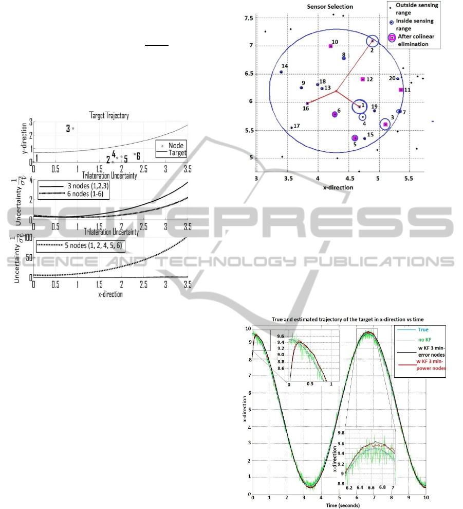
Figure 2: Trajectory of the target and distribution of the
sensor nodes.
4 NUMERICAL EXAMPLE
The following example used a sensor field of
dimensions 1010 units to demonstrate the
selection of a minimum number of sensor nodes and
implementation of distributed Kalman filter for target
tracking. Assume that 441 sensor nodes are randomly
deployed in this sensor field as shown in Figure 2.
The power consumption profile using in the
simulation was based on the analysis in (Watfa and
Commuri, 2006) even though our approach did not
depend on any specific hardware platform. Let
,
,
,
,
, and
be the
transmitting power, receiving power, active power,
sensing power, sleeping power, and computational
power respectively. Let
be the maximum
available power of a node. The normalized power
consumption in each operating mode is defined as
follows.
Sleeping mode:
/
.
Active mode:
/
.
Sensing mode:
)/
.
Master mode
/
where is the number of sensing
nodes
.
ICINCO2013-10thInternationalConferenceonInformaticsinControl,AutomationandRobotics
376
Let the measurement noise variance
=0.1, and the
state noise variance
0.005. Let the trilateration
constraint in equation (8) be 5
. The function
in (1) was chosen as
.
based on
power management strategy.
The target was assumed to move along a sinusoid
trajectory as shown in Figure 3. The sensing radius
was 1.4, and the simulation time was 10 seconds
Figure 3: Uncertainty of trilateration algorithm.
Coordinates of 6 sensor nodes from #1 to #6 are
0,
0
,
1.8,0
,
0.9,2.5
,
1.9,0.3
,
2.0,0.4
and 2.3, 0.6
relatively.
Figure 3 demonstrated the relationship between
uncertainty of trilateration algorithm and the spatial
distribution of sensor nodes. When all 6 nodes were
chosen, the uncertainty of trilateration was the
smallest. When 3 nodes (1, 2, 3) were chosen, the
uncertainty was bigger but still met the requirement
(smaller than 5
. However, 5 nodes (1, 2, 4,
5, 6) yielded a large trilateration uncertainty, and did
not meet the required tracking quality. Thus, to
improve the tracking quality and to reduce number of
active sensors, nodes at location (1, 2, 3) are
preferable.
The selection algorithm was shown in Figure 4.
The target were at (4.3, 6.2), and the sensing radius
was 2.0. Initially, 20 nodes within the sensing range
of the target were assumed to have uniformly random
residual power.
Figure 5 illustrates the overall tracking
performance along the x-direction, and the
performance was improved by using the Kalman
filter. The estimated error was initially high due to
large initial error (the true coordinates of the target
was at 9.5 in x-direction, but the initial value for the
filter was 8.0), but it reduced greatly after about 0.3
Figure 4: The sensor nodes represent by the dots. Radiuses
of small circles are proportional to the residual power of
sensor nodes. The squares represent the small group of
sensors left after running the collinear elimination process.
The sensors inside the big circle are able to sense the
target. Three sensors #1, #2, and #16 minimized the power
cost while still satisfying the required trilateration
uncertainty. Meanwhile, three sensors #1, #2, #3 yielded
the minimum power consumption cost, but did not meet
the trilateration uncertainty condition.
Figure 5: True and estimated trajectory of the target in x-
direction. Without using the Kalman filter, the tracking
error was high and fluctuated as shown in green line.
When the Kalman filters were used (black and red line),
the tracking errors were reduced. The red line was the
performance when three nodes (which minimized power
cost) were used. When three nodes (which minimized
trilateration uncertainty) were used for tracking (black
line), the tracking error is smaller and smother.
second. The tracking performance (in black solid
line) of three nodes (which resulted in minimum
EnhancingtheLifeTimeofaWirelessSensorNetworkinTargetTrackingApplications
377
trilateration uncertainty) was better the performance
of three nodes (red line) – which resulted in
minimum power consumption cost. However, as
shown in the Figure 5, the difference was not
significant.
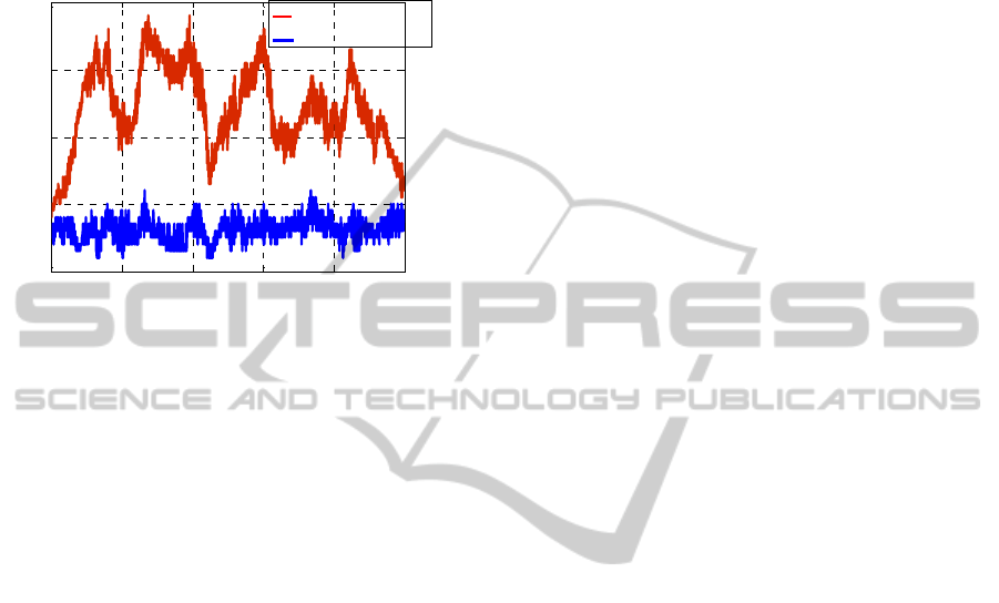
Figure 6: Number of sensed nodes before and after
collinear elimination.
In Figure 6, the average number of sensed nodes
before collinear elimination was 24.3, which resulted
in 2,529 exhaustive search attempts. After collinear
elimination process, only average 6.1 sensed nodes
remained, which the average total search attempts
reduced to 27.9 while the average actual search
attempts were 19.5.
5 DISCUSSION
5.1 Selection of the Power Cost
Function
In equation (1), power profile function
is a
decreasing continuous function and is selected by the
characteristic of a specific type of sensors and the
power management strategy. Different candidate of
can result in different set of chosen sensor
nodes, but nodes with more residual power are still
preferable over nodes that power is almost depleted.
Hence, the life time of the sensor network is
improved.
5.2 Selection of the Master Node
In equation (10), if α is large, the weighted cost
depends more on the current residual power of the
sensor and its cost to transmit data to the network
sink. If 1, (or 0) the node with lowest
power consumption cost is selected, but it can be
outside the communication range of the target’s
sensed nodes in the next tracking interval. On the
other hand, if 0 (or 1), the selected master
node is in the heading of the target, but its residual
power may be almost depleted.
5.3 The Selection Algorithm
In worst case scenario, the calculation time of the
selection algorithm is equal to that of exhaustive
search. However, the proposed algorithm performs
better in practice.
6 CONCLUSIONS
In this paper, an algorithm was proposed to enhance
the life time of a WSN by solving an optimization
problem which minimized the power consumption
cost function under the constraint of tracking quality.
Simulation illustrated that the suboptimal solution
reduced both computational complexity and the
number of active sensor nodes. Nodes with more
residual power were preferred for power intensive
tasks while nodes with low residual power were
scheduled to sleep. The numerical examples show
that the validity of the proposed approach. The future
work will focus on the tracking problem in three-
dimensional coordinate system with rigorous
mathematical analysis.
ACKNOWLEDGEMENTS
The first author would like to thank Dr. Choon Yik
Tang for the discussion about optimization problems
and heuristic search.
REFERENCES
Atia, G. K., Veeravalli, V. V. & Fuemmeler, J. A. 2011.
Sensor Scheduling For Energy-Efficient Target
Tracking In Sensor Networks. Ieee Transaction On
Signal Processing, 59, 4923 - 4937
Cui, S., Xiao, J.-J., Goldsmith, A., Luo, Z.-Q. & Poor, V.
2007. Estimation Diversity And Energy Efficiency In
Distributed Sensing Ieee Transaction On Signal
Processing, 55, 4683 - 4695
Demigha, O., Hidouci, W. & Ahmed, T. 2012. On Energy
Efficiency In Collaborative Target Tracking In
Wireless Sensor Network: A Review Ieee
Communication Surveys And Tutorials, Pp, 1-13.
0 2 4 6 8 10
0
10
20
30
40
Time (seconds)
Number of sensed nodes
Number of sensed node before and after colinear elimination
Before colinear elimiation
After colinear elimination
ICINCO2013-10thInternationalConferenceonInformaticsinControl,AutomationandRobotics
378

Fang, B. T. 1986. Trilateration And Extension To Global
Positioning System Navigation. Journal Of Guidance,
Control, And Dynamics, 9, 715-717.
Fang, J. & Li, H. 2009. Ieee Transaction On Wireless
Communications, 8, 3822 - 3832
Fuemmeler, J. A., Atia, G. K. & Veeravalli, V. V. 2011.
Sleep Control For Tracking In Sensor Networks. Ieee
Transaction On Signal Processing, 59, 4354-4366.
Lin, J., Xiao, W., Lewis, F. & Xie, L. 2009. Energy-
Efficient Distributed Adaptive Multisensor For
Scheduling For Target Tracking In Wireless Sensor
Networks. Ieee Transaction On Instrumentation And
Measurement, 58, 1886 - 1896
Manolakis, D. E. 1996. Efficient Solution And
Performance Analysis Of 3-D Position Estimation By
Trilateration. Ieee Transaction On Aerospace And
Electronic Systems, 32, 1239-1248.
Masazade, E., Niu, R. & Varshney, P. K. 2012. Dynamic
Bit Allocation For Object Tracking In Wireless Sensor
Networks. Ieee Transaction On Signal Processing, 60,
5048 - 5063.
Mukherjee, K., Gupta, S., Ray, A. & Wettergren, T. A.
2011. Statistical-Mechanics-Inspired Optimization Of
Sensor Field Configuration For Detection Of Mobile
Targets. Ieee Transaction On Cybernetics, 41, 783 -
791.
Onel, T., Ersoy, C. & Delic, H. 2009. Information
Content-Based Sensor Selection And Transmission
Power Adjustment For Collaborative Target Tracking.
Ieee Transaction On Mobile Computing, 8.
Pattem, S., Poduri, S. & Krishnamachari, B. Energy-
Quality Tradeoffs For Target Tracking In Wireless
Sensor Networks. Ipsn'03 Proceedings Of The 2nd
International Conference On Information Processing
In Sensor Networks 2003 Palo Alto, Ca. 32-46.
Powers, J. W. 1966. Range Trilateration Error Analysis.
Ieee Transaction On Aerospace And Electronic
Systems, Aes-2, 572.
Thomas, F. & Ros, L. 2005. Revisiting Trilateration For
Robot Localization. Ieee Transaction On Robotics, 21,
93-101.
Watfa, M. K. & Commuri, S. Optimal Sensor Placement
For Border Perambulation. 2006 Ieee International
Conference On Control Applications, 2006 Munich,
Germany.
Yang, Z. & Liu, Y. 2008. Quality Of Trilateration:
Confidence-Based Iterative Localization. Ieee
Transaction On Parallel And Distributed Systems, 21,
631-640.
Zhao, F., Shin, J. & Reich, J. 2002. Information-Driven
Dynamic Sensor Collaboration. Ieee Signal
Processing Magazine,
19, 61-72.
EnhancingtheLifeTimeofaWirelessSensorNetworkinTargetTrackingApplications
379
