
Online Dynamic Smooth Path Planning for an Articulated Vehicle
Thaker Nayl, George Nikolakopoulos and Thomas Gustafsson
Control Engineering Group Department of Computer Science, Electrical and Space Engineering,
Lule˚a University of Technology, Lule˚a, Sweden
Keywords:
Articulated Vehicle, Path Planning, Obstacle Avoidance.
Abstract:
This article proposes a novel online dynamic smooth path planning scheme based on a bug like modified
path planning algorithm for an articulated vehicle under limited and sensory reconstructed surrounding static
environment. In the general case, collision avoidance techniques can be performed by altering the articu-
lated steering angle to drive the front and rear parts of the articulated vehicle away from the obstacles. In
the presented approach factors such as the real dynamics of the articulated vehicle, the initial and the goal
configuration (displacement and orientation), minimum and total travel distance between the current and the
goal points, and the geometry of the operational space are taken under consideration to calculate the update on
the future way points for the articulated vehicle. In the sequel the produced path planning is being online and
iteratively smoothen by the utilization of Bezier lines before producing the necessary rate of change for the
vehicle’s articulated angle. The efficiency of the proposed scheme is being evaluated by multiple simulation
studies.
1 INTRODUCTION
Recently, there have been significant advances in
designing automated articulated vehicles mainly for
their utilization in the mining industry, where the aim
has been the overall increase of the production, while
making the working conditions for the human opera-
tors safer (Scheding et al., 1999). In most of the cases,
these vehicles are remotely operated, while there is
a continuous trend for increasing the autonomy lev-
els, especially in the area of path planning and obsta-
cle avoidance as the vehicles need: a) to perceive the
changing environment, based on the onboard sensory
systems and b) autonomously plan their route towards
the final objective (Roberts et al., 2000).
For the classical task of path planning, with an
obstacle detection and avoidance capability, the sim-
plest technique to solve the problem is the altering of
the vehicle’s orientation, while predicting a non colli-
sion path, based on the vehicle’s kinematic model, the
sensing range and the safety range. In this approach a
finite optimal sequence of control inputs, according to
the initial vehicle position and the desired goal point
is being generated, which is able to take under consid-
eration positioning and measuring uncertainties, such
that the collision with any obstacle at a given future
time never occurs.
From another point of view, path planning can be
divided in two main categories according to the as-
sumptions of: a) global approaches where it is being
assumed that the map is a priori available, and b) a
partially known and reconstructed surrounding envi-
ronment based on reactive approaches, which utilizes
sensors like infrared, ultrasonic and local cameras.
Characteristic examples of the first case are the Road–
Map algorithm (Nilsson, 1969), the Cell Decomposi-
tion (Chazelle, 1987), the Voronoi diagrams (Guechi
et al., 2008), the Occupancy Grinds (Usher, 2006)
and the new Potential Fields techniques (Ge and Cui,
2000), while in most of the cases, a final step of
smoothing the produced path curvatures, by the uti-
lization of Bezier curves is being utilized (
ˇ
Skrjanc and
Klanˇcar, 2010).
For the second case of a partially known and on-
line reconstructed environment, the Bug family al-
gorithms are well known mobile vehicle navigation
methods for local path planning based on a minimum
set of sensors and with a decreased complexityfor on-
line implementation (Ng and Br¨aunl, 2007). One of
the most commonly utilized path planning algorithm
in this category is the Bug1 and Bug2 (Lumelsky and
Stepanov, 1986). Bug1 algorithm exhibits two behav-
iors; motion to goal with boundary following and a
corresponding hit point and leave point, while Bug2
algorithm presents similar behaviors like the Bug1 al-
gorithm, except from the fact that it tries to follow
177
Nayl T., Nikolakopoulos G. and Gustafsson T..
Online Dynamic Smooth Path Planning for an Articulated Vehicle.
DOI: 10.5220/0004438301770183
In Proceedings of the 10th International Conference on Informatics in Control, Automation and Robotics (ICINCO-2013), pages 177-183
ISBN: 978-989-8565-71-6
Copyright
c
2013 SCITEPRESS (Science and Technology Publications, Lda.)
the fixed line from a start point to the goal, during
obstacle avoidance. Other Bug algorithms that also
incorporate range sensors are TangentBug (Kamon
et al., 1998), DistBug (Kamon and Rivlin, 1997) and
VisBug (Lumelsky and Skewis, 1990). Tangent Bug
algorithm is an improvement of the Bug2 algorithm
since it is able to determine the shorter path to the
goal using a range sensor with a 360
o
infinite orien-
tation resolution. DistBug has a guaranteed conver-
gence and will find a path if one exists, while it re-
quires the perception of its own position, the goal po-
sition and the range sensory data (Buniyamin et al.,
2011). The VisBug algorithm, needs global informa-
tion to update the value of the minimum distance to
the goal point, during the boundary following and for
determining the completion of a loop during the con-
vergence to the goal. In all the presented path plan-
ning algorithms, the vehicle is being modeled as a
point within the world space, without any constraint
in the movements, while the actual kinematics of the
vehicle, which is important especially in the case of
non–holonomic vehicles are being neglected.
The novelty of this article stems from the proposal
of a new bug like path planning algorithm based on
the dynamic model of an articulated vehicle, which is
able to consider: a) the physical constraints of the ve-
hicle, b) proper obstacle detection and avoidance, and
c) smooth path generation based on an online Bezier
lines processing of the produced way points. In the
presented approach the solution to the path planning
problem is generated online, based on partial and on-
line sensory information of the vehicle’s surrounding
environment, while the path is being calculated by
solving the inverse kinematic problem of the articu-
lated vehicle or by calculating the optimal articulation
angle. Moreover, as in the case of all the exploration
and final goal seeking algorithms, it is assumed that
the vehicle is constantly aware of the final goal co-
ordinates. During the convergence to this goal and
based on the limited range sensing of the surrounding
environment, the vehicle is able to detect and avoid
obstacles, while continue converging to the optimum
goal. This approach is providing an online and sub
optimal solution, when compared with the global path
planning techniques, and it can be directly applied to
the case of articulated vehicles. As it has been applied
in the previous path planning algorithms for the case
of a priori known space configuration, in the proposed
scheme, the Bezier curves are being also utilized for
filtering the produced way points and thus guarantee
for an online smooth path planning due to the Bezier’s
line property of continuous higher-order derivatives.
The rest of the article is organized as it follows.
In Section 2 the model of the articulated vehicle and
the corresponding state space equations will be pre-
sented. In Section 3 the proposed novel scheme for
smooth path planning and obstacle avoidance based
on the articulated vehicle’s dynamics will be intro-
duced, while in Section 4 multiple simulation results
will be depicted that prove the efficacy of the path
planning scheme in different test cases. Finally, the
concluding remarks are provided in Section 5.
2 ARTICULATED VEHICLE
MODEL
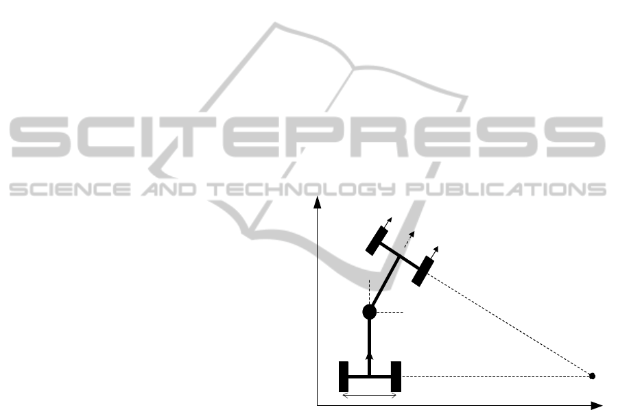
An articulated vehicle is constructed by two parts,
a front and a rear, linked with a rigid free joint,
while each body has a single axle and the wheels are
all non–steerable, with the steering action to be per-
formed on the joint, by changing the corresponding
articulated angle γ between the front and the rear of
the vehicle (Nayl et al., 2011) as it being also pre-
sented in Figure 1.
Y
X
P2=(X2,Y2)
v1
r1
r2
v2
Ө1
ϒ
l2
l1
Ө2
C
W
vL
vR
P1=(
X
1,
Y
1)
Figure 1: Articulated vehicle’s geometry.
The main assumptions to derive the kinematic
model of the articulated vehicle are: a) the steering
angle γ remains constant under small displacement,
b) dynamical effects due to low speed, like tire char-
acteristic, friction, load and breaking force are being
neglected, c) it’s assumed that the vehicle moves on a
plane without slipping effects, during low-level con-
trol, the vehicle’s velocities are bounded within the
maximum allowed velocities, which prevents the ve-
hicle from slipping, and c) each axle is composed of
two wheels and when replaced by a unique wheel, can
get:
˙
X
1
= V
1
cos θ
1
(1)
˙
Y
1
= V
1
sin θ
1
(2)
ICINCO2013-10thInternationalConferenceonInformaticsinControl,AutomationandRobotics
178
The steering angle γ is being defined as the difference
between the orientation angles of the front θ
1
and the
rear parts θ
2
of the vehicle.
The velocity V
1
at the front andV
2
at the rear parts
have the same changing with respect to the velocity at
the rigid free joint of the vehicle, and it can be defined
by the relative velocity vector equations as it follows:
V
1
= V
2
cos γ+
˙
θ
2
l
2
sinγ (3)
V
2
sinγ =
˙
θ
1
l
1
+
˙
θ
2
l
2
cos γ (4)
where
˙
θ
1
,
˙
θ
2
and l
1
, l
2
are the angular velocities and
the lengths of the front and rear parts of the vehicle
respectively. By combining these equations it yields:
˙
θ
1
=
V
1
sinγ+ l
2
˙
γ
l
1
cosγ+ l
2
(5)
while the angles γ and θ
1
can be measured with a
great accuracy. For the case that there is a steering
limitation for driving the rear part, according to the
coordinates of the point P
2
= (X
2
,Y
2
), the geometrical
relationship between P
1
and P
2
is provided by:
X
2
= X
1
− l
1
cosθ
1
− l
2
cosθ
2
(6)
Y
2
= Y
1
− l
1
sinθ
1
− l
2
sinθ
2
(7)
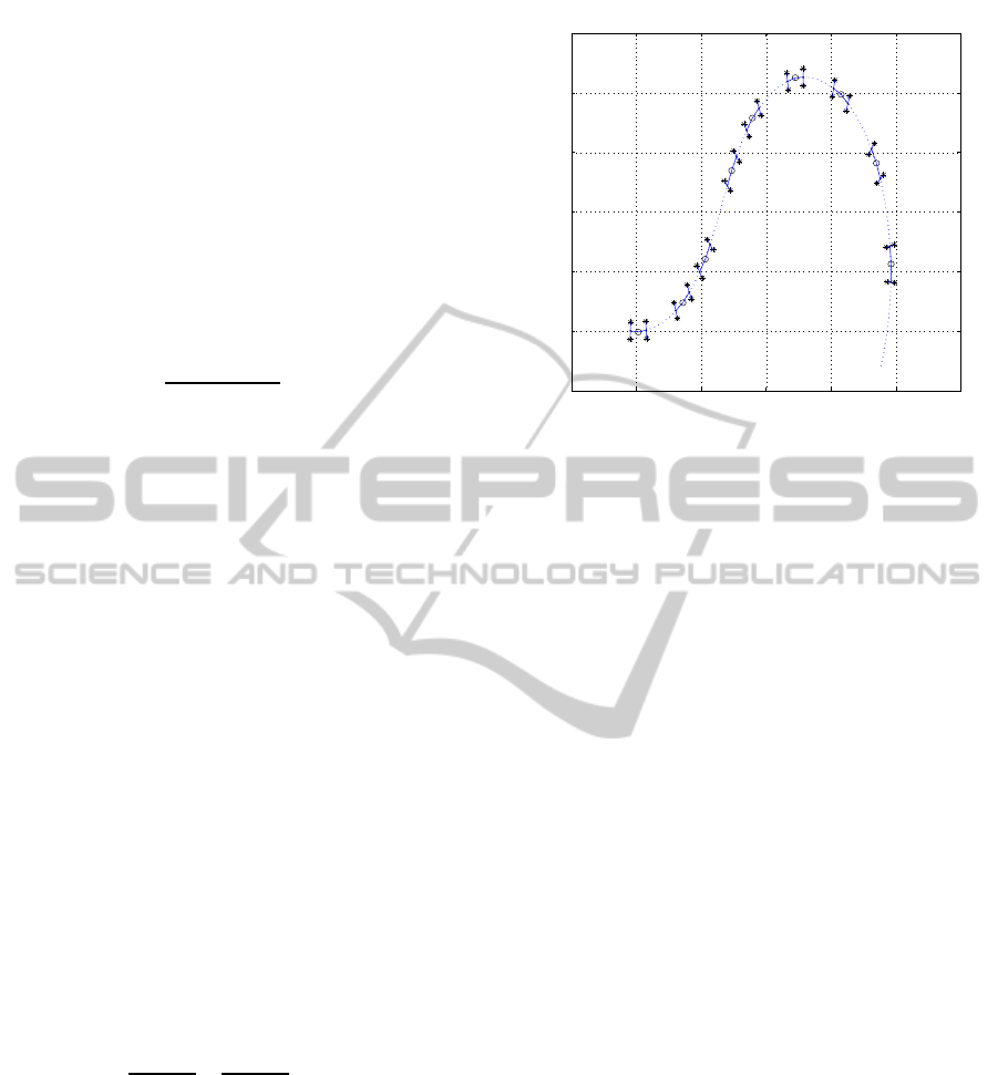
The realistic dynamic motion behavior of the articu-
lated vehicle with initial parameters [X
r
Y
r
θ
r
γ
r
], is
depicted in Figure 2, where the vehicle is requested to
reach the goal destination with a specific orientation.
As it can be observed, when the dynamics of the vehi-
cle are being incorporated the motion and the overall
behavior of the vehicle significantly deviates from the
case where the vehicle is being considered of having
the dynamics of an unconstraint point and this is one
of the major contributions of this article.
The state parameters of the articulated vehicle are;
X = [X Y θ γ]
T
and the manipulated variables are u =
[V
˙
γ]
T
, while the kinematic model of the articulated
vehicle, in a state space formulation can be written as
it follows:
˙
X
˙
Y
˙
θ
˙
γ
=
cosθ 0
sinθ 0
sinγ
l
1
cosγ+l
2
l
2
l
1
cosγ+l
2
0 1
V
˙
θ
γ
,
(8)
where
˙
θ
γ
is the rate of change for the articulated an-
gle.
3 ON LINE SMOOTH PATH
PLANNING FOR AN
ARTICULATED VEHICLE
The introduced path planning algorithm can be ap-
plied for the objective of moving a vehicle from a
−5 0 5 10 15 20 25
−2
0
2
4
6
8
10
X (m)
Y (m)
Start point
Reference path
Figure 2: Realistic dynamic motion behavior of the articu-
lated vehicle starting at [0 0 0 − 10
0
] with V = 1m/s and
˙
γ = 0
0
for the first 5sec of movement, while
˙
γ = 3.5
0
for
the next 6 sec to reach the goal point at [20 2]. The vehicle
dimensions are l
1
= l
2
= 0.6m and W = 0.58m.
starting point to the goal point, while detecting and
avoiding identified obstacles based on the real vehi-
cles dynamic equations of motion. As a common
property of the Bug like algorithms, the proposed
scheme initially faces the vehicle towards the goal
point, which it is being assumed to be a priori known.
In the proposed path planning module it is also be-
ing assumed that the vehicle is able to online sense
the surrounding environment based on the available
sensory systems. The proposed scheme is able to
replan the produced path, by generating new way
points, after the identification of an obstacle and pro-
duce proper path deformations that need to be done
for avoiding it. In all these cases the produced set
of new way points are utilized as control points for
a Bezier curve algorithm for online smoothing of the
suggested path. The overall proposed concept of the
novel path planning algorithm is being presented in
the following Figure 3.
As it can be observed from this diagram the algo-
rithm starts by defining the current position and orien-
tation of the vehicle, denoted by [X
r
, Y
r
, θ
r
] and the
final goal position denoted by [X
g
, Y
g
, θ
g
]. Based on
the onboard sensory system, the vehicle identifies the
surrounding environment and obstacles and generates
the way points for reaching the goal destination. In
the sequel the way points are been smoothen by the
utilization of Bezier filtering, while as a last step and
based on the vehicles dynamics, an open loop control
signal (articulated angle) is being generated to guide
the vehicle. In the presented approach it is also as-
sumed that the system is fully observable and good
and timely available measurements can be provided
OnlineDynamicSmoothPathPlanningforanArticulatedVehicle
179
Path
Planning
Obstacle
Avoidance
Algorithm
Smooth
Path
and Control
commands
Articulated
Vehicle
Range
Sensor
Initialization
Vehicle and
Target
Information
Xk
Yk
[dobs, Ɵobs]
+
Noise
+
[Xr Yr Ɵr]
[Xt Yt]
Current States [ΔX, ΔY, ΔƟ]
ɣ
Figure 3: Block diagram of the proposed path planning al-
gorithm based on the nonlinear articulated kinematic model.
for the displacement and orientation of the vehicle.
The assumed sensory system is able to detect the
obstacles and the surrounding environment, measure
the distance of the articulated robot from the obsta-
cle d
obs
∈ ℜ, while a sensing radius θ
obs
∈ ℜ is being
considered, reflecting real life sensing limitations. In
the presented approach all the obstacles and the sur-
rounding environment are being considered as point
clouds in a 2-dimensional space, while the overlap-
ping obstacles are being clustered and represented by
a single and unified obstacle.
Modefied path
Goal point
dobs
dw
Y
X
Өg
Өk
β
Өobs
Ө
min
d
min
v
Figure 4: Notations and overall concept of the proposed
path planning algorithm.
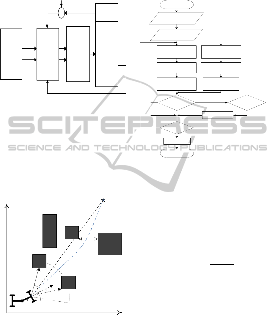
The overall flowchart diagram for path planning
and obstacle avoidance for the case of an articulated
vehicle is being depicted in Figure 5, while is can be
summarized as it follows:
[Step 1: Initialization] Define initial [X
r
Y
r
θ
r
˙
γ
r
] and
Start
Is the goal
reached?
End
Environment model,
range sensor
produce
(d
obs, Ɵobs)
Start motion by:
[X
k+1, Yk+1,Ɵk+1]=
[X
k, Yk,Ɵk]+
T*[ΔX, ΔY, ΔƟ]
Compute a new Ɵt,
β = Ɵ
g - Ɵk
[Xr, Yr,Ɵr]=[Xk, Yk,Ɵk]
change steering control
angle ɣ in smooth
movement using Bezier
curve
Any obstacle
around? d
obs ≤
safe range
Yes
No
Yes
Compute
[X
k+1, Yk+1,Ɵk+1]=
[X
k, Yk,Ɵk]+
T*[ΔX, ΔY, ΔƟ]
Small right or left
turn
No
Initiate robot and
goal parameters
[X
r, Yr,Ɵr, ɣ] and
[X
g, Yg]
Any obstacle
in front? Ɵ
obs ≤
safe angle
Yes
Judge right or left turn
according to Ɵ
obs and
duplicate β
No
Define robot’s
dynamics and
constraints
Set
Velocity=0
Figure 5: Main flowchart of path planning motion.
goal [X
g
Y
g
], define the articulated vehicle’s specific
parameters V, d
min
, θ
min
, d
obs
, θ
obs
, the path update
rate defined as T and the vehicle’s mechanical and
physical constraints that needs to be taken under con-
sideration. Set [X
k
Y
k
θ
k
] = [X
r
Y
r
θ
r
˙
γ
r
], with k ∈ Z
+
the sample index.
[Step 2: Path Update] Utilize Equations (1), (2), (6),
(7) and (8) to update the coordinates of the next way
point as:
[X
k+1
Y
k+1
θ
k+1
] = [X
k
Y
k
θ
k
] + T ∗ [∆X ∆Y ∆θ]
calculate:
θ
g
= arctan
Y
k+1
−Y
g
X
k+1
− X
g
β = θ
g
− θ
k
to produce γ with θ
g
the angle between the line that
connects the center of gravity of the vehicle’s front
part to the goal point and the X axis, while β is the
difference angle among the vehicle’s orientation an-
gle, with the X axis and θ
g
. During the application
of this step, constraints can be imposed on the artic-
ulated vehicle just by bounding the allowable articu-
lation within γ
+
≤
˙
γ ≤ γ
−
, with
+
and
−
representing
the maximum and the minimum bounds on the artic-
ulated angle.
[Step 3: Obstacle Avoidance] The obstacle avoid-
ance strategy becomes active when the safety condi-
tions d
min
and θ
min
are satisfied. This can be evaluated
ICINCO2013-10thInternationalConferenceonInformaticsinControl,AutomationandRobotics
180
by calculating the update of the distance from the ob-
stacle and the obstacle’s angle by:
Dis
obs
=
q
(X
k+1
− X
obs
)
2
+ (Y
k+1
−Y
obs
)
2
θ
obs
= arctan
Y
k+1
−Y
obs
X
k+1
− X
obs
θ
obs,g
= θ
obs
− θ
g
while in the case that the following conditions are
true:
(Dis
obs
< d
min
) AND (θ
obs,g
< θ
min
)
OR
(Dis
obs
< d
min
) AND (θ
obs,g
< −θ
min
)
the changing in the steering angle is being duplicated
and Step 3 is repeated again till the condition in (9) is
false and the algorithm continues from Step 2 or the
bounds on the articulated angle cannot meet and the
algorithm jumps to Step 4.
[Step 4: Reaching Final Goal] If [X
k+1
Y
k+1
] =
[X
g
Y
g
] ± Dis
tolr
, set velocity = 0 and the path plan-
ning algorithm has been terminated. Otherwise, the
algorithm jumps to Step 2 and the whole process is
being repeated in order to avoid collisions with the
obstacles until vehicle reaches the goal tolerance dis-
tance.
During the execution of the proposed path plan-
ning algorithm, and especially Step 2, the proposed
path planning algorithm always smoothes the pro-
duced way points by the utilization of Bezier curve
filtering. The mathematical formulation of the applied
Bezier smothering is denoted as:
B(t) =
n
∑
i=0
(
n
i
) (1− t)
n−i
t
i
P
i
, t ∈ [0,1] (9)
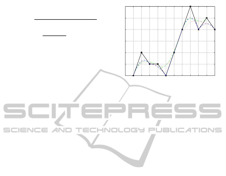
The number n of the considered control points for the
Bezier curve generation plays a significant role in the
final shape of the produced smooth path as it can be
observed from Figure 6, where multiple Bezier lines
are being displayed with respect to different num-
ber of control points. A n degree Bezier line always
passes through the first and last control points and it
can be provedthat it alwayslies within the convexhull
of the control points, while being tangent to the lines
connecting the way points (Chaudhry et al., 2010).
4 SIMULATION RESULTS
For simulating the efficacy of the proposed path plan-
ner, the following articulated vehicle’s characteristics
have been considered: l
1
= l
2
= 0.6m, W = 0.58m,
while the vehicle’s speed is constant and equal to
0 1 2 3 4 5 6 7 8 9 10 11
1
2
3
4
5
6
7
X (m)
Y (m)
Figure 6: Bezier curves based on different number of con-
trol points resulting in different paths, (Black line-solid path
produced from the generated way points, red line-dots for 6
points, green line-dash dot for 4 points and the blue line-
dash for 3 points).
1msec. Moreover, the constraints imposed on the ar-
ticulated angle γ have been defined as ±0.523 rad
and random measurement Gaussian noise with a fixed
variance was added to all measurements of the range
sensor to simulate the real life measurement distor-
tion.
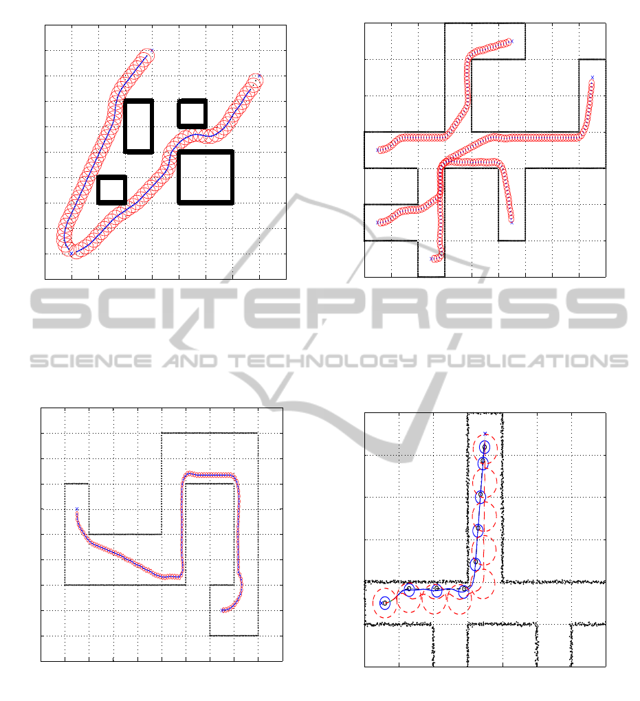
The effectiveness of the proposed algorithm will
be evaluated in arenas of different types and dimen-
sions. More analytically, the algorithm is simulated
on three types of environments with different obsta-
cle configurations, where the vehicle and obstacle ge-
ometry is described in a 2D workspace. The obtained
outputs of the path planning solutions from the indi-
cated starting points to the goal points is being de-
picted in Figures 7, 8 and 9, displaying cases with the
same sensing radius d
obs
= 3m and various d
min
.
As it can be observed in all the examined cases
the vehicle is able to avoid all the obstacles, includ-
ing the bounding surrounding (e.g. walls), which can
also be considered as obstacles without loss of gener-
ality. In the presented simulations, the articulated ve-
hicle is achieving to reach the reference final goal, in-
dependently of the initial vehicle’s orientation, while
in all the simulations the safety radius has been also
displayed with the red circle notation. The basic as-
sumption in all these simulations is that the articu-
lated vehicle, in every time instant, is aware of the
coordinates of the final goal and thus the path is being
tuned in every step based on the identified obstacles,
while the vehicle explores the surrounding environ-
ment towards the final goal. In an obstacle free envi-
ronment, the optimal solution to this problem would
have been a straight line connecting the initial with
the goal point, a case that can be easily identified in
the presented simulation in Figure 7. The online iden-
OnlineDynamicSmoothPathPlanningforanArticulatedVehicle
181
−5 0 5 10 15 20 25 30 35 40
−5
0
5
10
15
20
25
30
35
40
45
X (m)
Y (m)
Goal point 1
Goal point 2
Figure 7: Different shape obstacles placed in the workspace.
During these simulations the vehicle starts from different
initial angles at [0, 0, 120
0
, 7.5
0
] and [0, 0, 20
0
, 7.5
0
] to
reach the goal points located at [15, 40] and [35, 35] respec-
tively, with safe distance d
min
= 3m, d
obs
= 3m.
−10 0 10 20 30 40 50 60 70 80 90
−5
0
5
10
15
20
25
30
35
40
45
X (m)
Y (m)
Start point
Goal point
Figure 8: Path planning in an arena having boundaries on
both sides of the road a fact that restricts the articulated ve-
hicle motions. During this simulation scenario the vehicle
is starting from the initial posture [5, 25, − 90
o
, 7.5
o
] and
the goal is located at [65, 5] and d
min
= 0.5m, d
obs
= 3m.
tification of obstacles produces distortions from fol-
lowing the straight line, connecting the robot with the
final goal point, while the sensing and safety radius
are having a major effect on the path calculation. As
it can observed in Figure 10, the safety radius plays a
very significant role in shape of the path. In this Fig-
10 20 30 40 50 60 70 80 90 100
10
20
30
40
50
60
70
80
X (m)
Y (m)
Start point 3
Goal point 3
Start point 2
Start point 1
Goal point 1
Goal point 2
Figure 9: Path planning in an arena having more compli-
cated boundaries on both sides of the road, with noise mea-
surement. The scenario is starting from different initial pos-
tures [15, 45], [15, 25] and [35, 15] with initial [θ, γ] =
[10
o
, 7.5
o
] and the goals are located at [65, 75], [95, 65]
and [65, 25] respectively with d
min
= 1.0m, d
obs
= 3m.
10 20 30 40 50 60 70 80
30
40
50
60
70
80
90
X (m)
Y (m)
Start point
Goal
point
Figure 10: During these simulations the vehicle is starting
from the initial posture [15, 45, 0, 5
0
] and the goal point
is located at [45, 85], while during movement different safe
distances d
min
have been utilized as 0.5, 1.5 and 3.5m, with
the same d
obs
= 3m.
ure, different paths with different safe distances d
min
and with the same sensing radius d
obs
are being pre-
sented. In the case that the vehicle is moving in a
bounded space, the selection of a relatively big safety
radius introduces oscillations in the translation of the
robot due to sequential safety violations that produce
ICINCO2013-10thInternationalConferenceonInformaticsinControl,AutomationandRobotics
182

corresponding change in the direction of the vehicle
for avoiding the obstacle. In case that small safety ra-
dius are being selected, this effect is being vanished
and smooth and shorter, non oscillatory, paths can be
produced.
Finally it should be stated that the arenas in Fig-
ures 8 and 9 are typical realistic examples of areas
where articulated vehicles operate, as the mine tun-
nels and the civil roads are. In the presented simu-
lations the consideration of the articulated vehicle’s
dynamic motion is obvious especially in the time in-
stances where the vehicle is turning towards the goal
and while performing at the same time obstacle avoid-
ance. This effect is of paramount importance for the
case of articulated vehicles as classical point dynamic
approaches in path planning will obviously results in
non-realistically achievable paths that would directly
lead to collisions.
5 CONCLUSIONS
In this article a novel online dynamic smooth path
planning scheme based on a bug like modified path
planning algorithm for an articulated vehicle under
limited and sensory reconstructed surrounding static
environment has been proposed. In the presented ap-
proach factors such as the real dynamics of the ar-
ticulated vehicle, the initial and the goal configura-
tion, the minimum and total travel distance between
the current and the goal points, the geometry of the
operational space, and the path smothering approach
based on Bezier lines have been taken under consider-
ation to produce a proper path for an articulated vehi-
cle, which can be followed by correspondingly alter-
ing the vehicle’s articulated angle. The efficiency of
the proposed scheme has been evaluated by multiple
simulation studies.
REFERENCES
Buniyamin, N., Wan Ngah, W., Sariff, N., and Mohamad,
Z. (2011). A simple local path planning algorithm
for autonomous mobile robots. International journal
of systems applications, Engineering & development,
5(2):151–159.
Chaudhry, T., Gulrez, T., Zia, A., and Zaheer, S. (2010).
B´ezier curve based dynamic obstacle avoidance and
trajectory learning for autonomous mobile robots. In
Intelligent Systems Design and Applications (ISDA),
2010 10th International Conference on, pages 1059–
1065. IEEE.
Chazelle, B. (1987). Approximation and decomposition of
shapes. Advances in Robotics, 1:145–185.
Ge, S. and Cui, Y. (2000). New potential functions for mo-
bile robot path planning. Robotics and Automation,
IEEE Transactions on, 16(5):615–620.
Guechi, E., Lauber, J., and Dambrine, M. (2008). On-line
moving-obstacle avoidance using piecewise bezier
curves with unknown obstacle trajectory. In Control
and Automation, 2008 16th Mediterranean Confer-
ence on, pages 505–510. IEEE.
Kamon, I., Rimon, E., and Rivlin, E. (1998). Tangentbug:
A range-sensor-based navigation algorithm. The In-
ternational Journal of Robotics Research, 17(9):934–
953.
Kamon, I. and Rivlin, E. (1997). Sensory-based motion
planning with global proofs. Robotics and Automa-
tion, IEEE Transactions on, 13(6):814–822.
Lumelsky, V. and Skewis, T. (1990). Incorporating
range sensing in the robot navigation function. Sys-
tems, Man and Cybernetics, IEEE Transactions on,
20(5):1058–1069.
Lumelsky, V. and Stepanov, A. (1986). Dynamic path plan-
ning for a mobile automaton with limited information
on the environment. Automatic Control, IEEE Trans-
actions on, 31(11):1058–1063.
Nayl, T., Nikolakopoulos, G., and Guastafsson, T. (2011).
Kinematic modeling and simulation studies of a lhd
vehicle under slip angles. In Computational Intelli-
gence and Bioinformatics/755: Modelling, Identifica-
tion, and Simulation. ACTA Press.
Ng, J. and Br¨aunl, T. (2007). Performance comparison of
bug navigation algorithms. Journal of Intelligent &
Robotic Systems, 50(1):73–84.
Nilsson, N. (1969). A mobile automaton: An application
of artificial intelligence techniques. Technical report,
DTIC Document.
Roberts, J., Duff, E., Corke, P., Sikka, P., Winstanley, G.,
and Cunningham, J. (2000). Autonomous control of
underground mining vehicles using reactive naviga-
tion. In Robotics and Automation, 2000. Proceed-
ings. ICRA’00. IEEE International Conference on,
volume 4, pages 3790–3795. IEEE.
Scheding, S., Dissanayake, G., Nebot, E., and Durrant-
Whyte, H. (1999). An experiment in autonomous nav-
igation of an underground mining vehicle. Robotics
and Automation, IEEE Transactions on, 15(1):85–95.
ˇ
Skrjanc, I. and Klanˇcar, G. (2010). Optimal cooperative
collision avoidance between multiple robots based on
bernstein–b´ezier curves. Robotics and Autonomous
systems, 58(1):1–9.
Usher, K. (2006). Obstacle avoidance for a non-holonomic
vehicle using occupancy grids. In 2006 Australasian
Conference on Robotics and Automation.
OnlineDynamicSmoothPathPlanningforanArticulatedVehicle
183
