
Selecting Adequate Samples for Approximate Decision Support
Queries
Amit Rudra
1
, Raj P. Gopalan
2
and N. R. Achuthan
3
1
School of Information Systems, Curtin University, Ken Street, Bentley WA 6102, Australia
2
Department of Computing, Curtin University, Ken Street, Bentley WA 6102, Australia
3
Department of Mathematics and Statistics, Curtin University, Ken Street, Bentley WA 6102, Australia
Keywords: Sampling, Approximate Query Processing, Data Warehousing, Inverse Simple Random Sample without
Replacement (SRSWOR).
Abstract: For highly selective queries, a simple random sample of records drawn from a large data warehouse may not
contain sufficient number of records that satisfy the query conditions. Efficient sampling schemes for such
queries require innovative techniques that can access records that are relevant to each specific query. In
drawing the sample, it is advantageous to know what would be an adequate sample size for a given query.
This paper proposes methods for picking adequate samples that ensure approximate query results with a
desired level of accuracy. A special index based on a structure known as the k-MDI Tree is used to draw
samples. An unbiased estimator named inverse simple random sampling without replacement is adapted to
estimate adequate sample sizes for queries. The methods are evaluated experimentally on a large real life
data set. The results of evaluation show that adequate sample sizes can be determined such that errors in
outputs of most queries are within the acceptable limit of 5%.
1 INTRODUCTION
Decision support queries often involve applying
aggregate functions like count, average, and sum on
relatively small subset of records in a data
warehouse. Approximate results are usually
sufficient for such queries to provide a good idea of
how a business is doing. While relatively small
random samples can be used effectively for some
data warehouse queries, they are not suitable for
highly selective queries as the records that satisfy
the query conditions may not be adequately
represented in such samples. Ideally, an adequate
sample for such a query should be drawn from a
subset of the data warehouse that satisfies the
query’s selection conditions. A sample is adequate
for a query if it can be used to estimate the query
result with its accuracy within a specified confidence
interval. In this paper, we focus on estimating the
sizes of adequate samples for specific queries.
As Olken and Rotem (1990) pointed out, picking
records at random from a database without prior
rearrangement is very inefficient since a large
number of disk accesses may be needed to retrieve a
sample. To alleviate this problem, several recent
schemes for approximate query processing have
been proposed (Aouich and Lemire 2007); (Heule et
al., 2013); (Jermaine 2007); (Jermaine 2003);
(Jermaine et al., 2004); (Jin et al., 2006); (Joshi and
Jermaine, 2008); (Li et al., 2008); (Spiegel and
Polyzotis, 2009). Joshi and Jermaine (2008)
introduced the ACE Tree, which is a binary tree
index structure for efficiently drawing samples for
processing database queries. They demonstrated the
effectiveness of this structure for single and two
attribute database queries, but did not deal with
multi-attribute aggregate queries. For extending the
ACE Tree to k key attributes, Joshi and Jermaine
(2008) proposed binary splitting of one attribute
range after another at consecutive levels of the
binary tree starting from the root; from level k+1,
the process is repeated with each attribute in the
same sequence as before. This process could lead to
an index tree of very large height for a data
warehouse even if only a relatively small number of
attributes are considered. Rudra et al., (2012)
proposed the k-MDI Tree, that extends the ACE
Tree structure to deal with multi-dimensional data
warehouses with k-ary splits of data ranges. It was
shown that random samples of relevant rows (rows
46
Rudra A., P. Gopalan R. and R. Achuthan N..
Selecting Adequate Samples for Approximate Decision Support Queries.
DOI: 10.5220/0004444200460055
In Proceedings of the 15th International Conference on Enterprise Information Systems (ICEIS-2013), pages 46-55
ISBN: 978-989-8565-59-4
Copyright
c
2013 SCITEPRESS (Science and Technology Publications, Lda.)

that satisfy the conditions of a given query) could be
drawn more efficiently using the k-MDI tree.
The sampling scheme using the k-MDI tree index
(Rudra et al., 2012) facilitates picking rich samples
for queries with highly specific selection conditions.
If the sample contains an adequate number of
records that satisfy the query conditions, the average
values can be estimated from these records.
However, to estimate sum (= avg
x count) we need
to estimate both the average as well as count of the
records that satisfy the query in the whole database.
Therefore, from the sample we need to project the
number of records in the entire database that satisfy
the given query conditions. Chaudhuri and Mukerjee
(1985) proposed an unbiased estimator based on
inverse simple random sampling without
replacement (SRSWOR) where random sampling is
carried out on a finite population until a predefined
number of domain members are observed. In this
paper, we propose the adaptation of inverse
SRSWOR to estimate adequate sample sizes for
queries using the k-MDI tree index. The method is
empirically evaluated on a large real world data
warehouse.
The rest of the paper is organized as follows: In
Section 2, we briefly describe the k-way multi-
dimensional (k-MDI) indexing structure and the
storage structure of data records. Section 3 discusses
how to pick adequate samples using inverse
SRSWOR. In Section 4 we discuss the results of our
experiments. Finally, Section 5 concludes the paper.
2 TERMS, DEFINITIONS AND
k-MDI TREE INDEX
In this section, we define some terms pertaining to
data warehousing, define confidence interval and
then review the k-MDI tree index for retrieving
relevant samples from a data warehouse.
2.1 Dimension and Measures
To execute decision support queries, data is usually
structured in large databases called data warehouses.
Typically, data warehouses are relational databases
with a large table in the middle called the fact table
connected to other tables called dimensions. For
example, consider the fact table
Sales shown as Table
1. A dimension table
Store linked to StoreNo in this
fact table will contain more information on each of
the stores such as store name, location, state, and
country (Hobbs et al., 2003). Other dimension tables
could exist for items and date. The remaining
attributes like quantity and amount are typically, but
not necessarily, numerical and are termed measures.
A typical decision support query aggregates a
measure using functions such as Sum(), Avg() or
Count(). The fact table Sales along with all its
dimension tables forms a star schema.
Table 1: Fact table SALES.
SALES
StoreNo Date Item Quantity Amount
21 12-Jan-11 iPad 223 123,455
21 12-Jan-11 PC 20 24,800
24 11-Jan-11 iMac 11 9,990
77 25-Jan-11 PC 10 12,600
In decision support queries a measure is of
interest for calculation of averages, totals and
counts. For example, a sales manager may like to
know the total sales quantity and amount for certain
item(s) in a certain period of time for a particular
store or even all (or some) stores in a region. This
may then allow her to make decisions to order more
or less stocks as appropriate at a point in time.
2.2 Multidimensional Indexing
The k-ary multi-dimensional index tree (k-MDI tree)
proposed in Rudra et al., (2012) extends the ACE
Tree index (Joshi and Jermaine, 2008) for multiple
dimensions. The height of the k-MDI tree is limited
to the number of key attributes. As a multi-way tree
index, it is relatively shallow even for a large
number of key value ranges and so requires only a
small number of disk accesses to traverse from the
root to the leaf nodes.
The k-MDI tree is a k-ary balanced tree (Bentley
1975) as described below:
1. The root node of a k-MDI tree corresponds to the
first attribute (dimension) in the index.
2. The root points to k
1
(k
1
≤ k) index nodes at level
2, with each node corresponding to one of the k
1
splits of the ranges for attribute a
1
.
3. Each of the nodes at level 2, in turn, points to up
to k
2
(k
2
≤ k) index nodes at level 3
corresponding to k
2
splits of the ranges of values
of attribute a
2
; similarly for nodes at levels 3 to
h, corresponding to attributes a
3
,..., a
h
.
4. At level h, each of up to k
h-1
nodes points to up to
k
h
(k
h
≤ k) leaf nodes that store data records.
5. Each leaf node has h+1 sections; for sections 1 to
h, each section i contains random subset of
records in the key range of the node i in
SelectingAdequateSamplesforApproximateDecisionSupportQueries
47

Figure 1: General structure of the k-MDI tree.
the path from the root to the level h above the
leaf; section h+1 contains a random subset of
records with keys in the specific range for the
given leaf.
Thus, the dataset is divided into a maximum of k
h
leaf nodes with each leaf node, in turn, consisting of
h+1 sections and each section containing a random
subset of records. The total number of leaf nodes
depends on the total number of records in the dataset
and the size of a leaf node (which may be chosen as
equal to the disk block size or another suitable size).
More details on leaf nodes and sections are given in
sub-section II.C. In real data sets, the number of
range splits at different nodes of a given level i need
not be the same. For convenience, the number of
splits at all levels are kept as k in Figure 1 that
shows the structure of the general scheme for k-MDI
multilevel index tree of attributes A
1
, A
2
, …, A
h
with
k ranges (R
11
, R
12
, …, R
1k
), (R
21
, R
22
, …, R
2k
), …
(R
h1
, R
h2
, …, R
hk
) respectively at levels (1, …, h). In
other words,
R
ij
is the i-th attribute’s j-th range high
water mark (HWM).
An example of the k-MDI tree is shown in Figure
1 from a store chain dataset with three dimensions –
store, date sold and item number. The number of
range splits and hence branches from non-leaf nodes
vary between 2 and 4 in this example.
2.3 Leaf Nodes
The lowest level nodes of a k-MDI tree point to leaf
nodes containing data records. The data records are
stored in h+1 sections, where h is the height of the
tree. Section S
1
of every leaf node is drawn from the
entire database with no range restriction on the
attribute values. Each section S
i
(2 ≤ i ≤ h+1) in a
leaf node L is restricted on the range of key values
by the same restrictions that apply to the
corresponding sub-path along the path from the root
to L. Thus for section S
2
, the restrictions are the
same as on the branch to the node at level 2 along
the path from the root to L and so on.
Figure 2 shows an example leaf node projected
from the sample k-MDI tree. The sections are
indicated above the node with attribute ranges for
each section below the node. The circled numbers in
each section indicate record numbers that are
randomly placed in the section. The range
restrictions on the records are indicated below each
section, where the first section S
1
has records drawn
from the entire range of the database. Thus, it can
contain records uniformly sampled from the whole
dataset. The next section S
2
has restriction on the
first dimension viz. store (for leaf node L
7
this range
is store numbers 1-16). The third section S
3
has
restrictions on both first and second dimensions viz.
store and date. While the last section S
4
has
restrictions on all the three dimensions – store, date
and item.
The scheme for selection of records into various
leaf nodes and sections is explained in detail in the
following section.
2.4 Using the k-MDI Tree for Data
Warehouse Queries
By using a k-MDI tree index, we can draw stratified
samples for data warehousing queries from restricted
A
1
A
2
. . .
A
h
R
11
R
12 . . .
R
1k
Leaf nodes
. . .
Index tree
A
1
A
2
... A
h-1
A
h
R
11
R
21
R
h- 1 1
R
h1
R
h2 …
R
hk
A
1
A
2
... A
h
R
11
R
21
R
22 …
R
2k
A
1
A
2
... A
h
R
12
R
21
R
22 …
R
2k
A
1
A
2
... A
h
R
1k
R
21
R
22 …
R
2k
... ... .... . .
.
.
.
.
.
.
. . .
A
1
A
2
... A
h-1
A
h
R
11
R
21
R
h- 1 2
R
h1
R
h2 …
R
hk
. . .
A
1
A
2
... A
h-1
A
h
R
1k
R
2k
R
h- 1 k
R
h1
R
h2 …
R
hk
...
...
... ...
. . .
...
Level 1-Dim A
1
Level 2-Dim A
2
Level h-Dim A
h
.
.
ICEIS2013-15thInternationalConferenceonEnterpriseInformationSystems
48
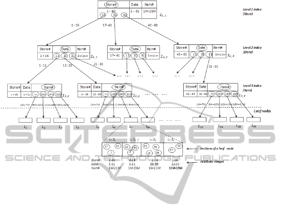
Figure 2: A leaf node (changes in range values for attributes are indicated in bold).
ranges of key values. The database relevancy ratio
(DRR) of a query Q, denoted by ρ(Q) is the ratio of
the number of records in a dataset D that satisfies the
query conditions to the total number of records in D.
For a query with no condition, ρ(Q) is 1. Similarly,
the sample relevancy ratio (SRR) of a query Q for a
sample set S, denoted by ρ(Q, S) is defined as the
ratio of the number of records in S that satisfy a
given query Q to the total number of records in S.
In a true random sample of records, the SRR for
a query Q is expected to be equal to its DRR, i.e.,
E(ρ(Q, S) ) = ρ(Q). A sample with ρ(Q, S) > ρ(Q) is
likely to give a better estimate of the mean than a
true random sample. However, for the sum of a
column, the sample needs to be representative of the
population, i.e., ρ(Q, S) should be close to ρ(Q).
Consider the following formula for estimating
the sum (Berenson and Levine 1992):
̂
,
where N is the cardinality of the population, ̂ the
estimated proportion of records satisfying the query
conditions and
the mean of records in the sample
satisfying the query condition. In order to estimate
the mean we can use all relevant sampled records
from all sections of the retrieved leaf nodes, but to
estimate the sum we can use sampled records only
from section S
1
, which is the only section with
records drawn randomly from the entire dataset. For
estimating the sum for a query with conditions on
some of the indexed dimensions we use appropriate
sections of the retrieved leaf nodes to get a better
estimate of the mean; the records from section S
1
are
used to get a fair estimation of the proportion of
records that satisfy the query conditions.
2.5 Effect of Sectioning on Relevancy
Ratio
As discussed earlier, sections S
1
to S
h+1
of each leaf
node contain random collections of records with the
difference that S
1
contains records from the entire
dataset while other sections contain random records
from restricted ranges of the key attributes. Consider
a query with the same range restrictions on all three
dimensions (store, date and item) as section L
7
.S
4
in
Figure 2. We are then likely to get more relevant
records in the sample from the second section L
7
.S
2
than from S
1
since records of S
2
have restrictions on
the first dimension of store that matches the query
condition. Records in S
3
will have restrictions on
both store and date dimensions that match that of the
query and so likely to contain more relevant records
than in S
2
. All records in section L
7
.S
4
will satisfy the
query since the range restrictions on S
4
exactly
match the query. Mathematically, for a query Q
having restrictions as mentioned above:
SelectingAdequateSamplesforApproximateDecisionSupportQueries
49

ρ(Q) = E(ρ(Q, L
7
.S
1
)) ≤ E(ρ(Q, L
7
.S
2
))
≤ E(ρ(Q, L
7
.S
3
)) ≤ E(ρ(Q, L
7
.S
4
))
Using this property of the k-MDI tree, it is possible
to quickly increase the size of a sample that is too
small, by including more records from other sections
of the retrieved leaf nodes.
2.6 Record Retrieval to Process a
Query
The objective of using the k-MDI tree is to retrieve a
significant number of relevant records (i.e. records
that satisfy the query conditions) in the sample
drawn for processing a given query. The query
conditions may span sections of one or more leaf
nodes, which can be reached from index nodes that
straddle more than one range of attribute values.
Traversing the tree from the root using the attribute
value ranges in the query conditions can access these
leaf nodes. Sections from multiple leaf nodes are
then combined to form the sample.
We describe the retrieval process using an
example query on the sample database of Figure 2.
Consider a query Q
0
about sales in store 12 for date
range 1-13 and item range 12M-20M. The retrieval
algorithm finds the sections of leaf nodes for this
query as follows:
1. Search index level 1 to locate the relevant store
range. Store 12 is in the left most range of 1-16.
2. Traverse down to index level 2 (date), indicated
by a dashed arrow in Figure 3, along the first
store range. Since there is a condition on date (1-
13), compare the HWMs (high water marks) of
the three ranges and find that it fits into two date
ranges viz. the first and the second. Make a note
of these date ranges.
3. Traverse down using the first date range to the
next index level, which has item ranges. Since
there is a condition on item numbers (12M-
20M), compare this range with HWMs and find
that it fits into two ranges viz. the third and the
fourth. Make a note of these item ranges.
4. Traverse down using the third item range to
relevant leaf pages and make a note of them.
5. Iterate step 4, except this time using the fourth
item range.
6. Next, repeat the above three steps i.e. steps 3
through 5; but this time using the second date
range instead.
7. Now retrieve records from the relevant sections
in the four leaf nodes (viz. L
3
, L
4
, L
7
and L
8
) to
form a sample for the given query.
3 SAMPLING TO ADEQUATE
LEVELS USING INVERSE
SRSWOR
An important question to be answered is how much
sampling is adequate to estimate some property of a
population. For business analytics on very large data
(Chaudhuri, 2012), it is valuable to provide the
analytic query user with incremental feedback of the
ongoing progress of an approximate query (Fisher
2011); (Fisher et al., 2012). The method described
below for determining if an adequate sample size
has been retrieved is based on the works of
Chaudhuri and Mukerjee (1985) and Sangngam and
Suwatee (2010). Their research established that
inverse simple random sampling without
replacement (or inverse SRSWOR) method provides
an unbiased estimate of the number of data points
(M) satisfying property P, if sampling is continued
until a pre-assigned number, say m, of data points
satisfying property P are present in the sample. In
the present case, property P would be the conditions
imposed on a query viz. the dimension ranges. For a
given query Q, assume that we have determined the
estimate of
()Q
.
Recall that
We could also choose the above sample size n as
follows:
Fix the error we are ready to tolerate, say e. Then
choose
2
/2
2
()(1 ())zQ Q
n
e
, where e is a number
such as 0.01, 0.02, or 0.05 etc. and
/2
z
is the
normal ordinate such that
/2
Prob P(Q)>
2
z
where P(Q) is the random variable representing ρ(Q).
Usually we take
= 0.05
for 95% confidence
interval.
Now estimate ρ(Q) again using this new sample
size. Henceforth, assume that we have this new
estimate with error bounded by e. In fact, when the
true value of ρ(Q) is not too close to zero (0) or one
(1), and sample size n is large enough we know that
the random variable P(Q) representing ρ(Q), follows
approximately the Normal distribution with mean
()Q
and standard deviation
()(1 ())
.
QQ
n
. Now
assume that the true value of
()Q
is not too close to
zero (0) or one (1), then we can get 95% confidence
interval for true value of ρ(Q) as
Number of cases satisying conditions of query Q
() .
sample size n
Q
ICEIS2013-15thInternationalConferenceonEnterpriseInformationSystems
50
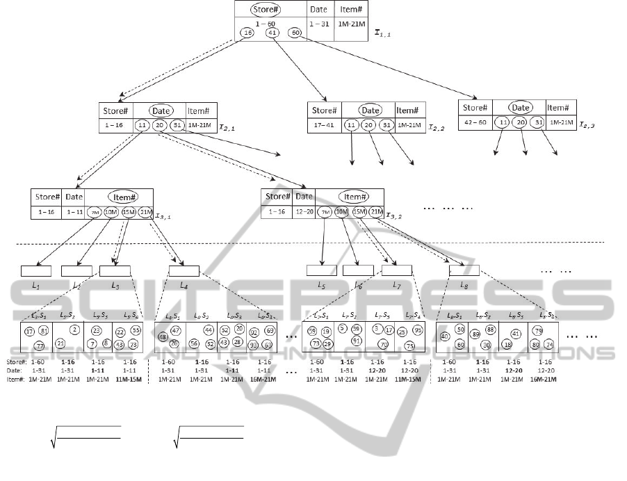
Figure 3: Navigation down index tree nodes for conditions on three dimensions.
( )(1 ( )) ( )(1 ( ))
()1.96 ,() 1.96 ,
QQ QQ
QQ
nn
(1)
Using the confidence interval (1) we can choose
about 5 to 10 possible values for P(Q). These values
may correspond to 10, 25, 50, 75, 90 percentile
points of the random variable P(Q). Let us denote
these values by .
Using these 5 percentiles, choose 10% or 20% of
the corresponding M values as possible choice of
values for m. More specifically,
;
;
;
;
and
.
Henceforth, denote these 10 possible values of m by
m
t
, 1≤ t ≤ 10. We now describe the Basic Find_M or
BF_M algorithm and the steps involved. There are
five steps in the BF_M algorithm, which are as
follows:
1. Initialization: In this step, various variables, like
counts and cumulative totals, are initialized.
2. Sampling: Records are sampled iteratively and
those meeting the given condition i.e. satisfying the
given property, say P, are used for calculating the
sum and the count of the value(s) in the query.
3. Check & Iterate: This step checks if adequate
number of samples have been retrieved. In case, it
has not reached the targeted number of samples, it
iterates the sampling step, else it terminates further
sampling.
4. Estimation: In this step, unbiased estimators of
M, average and sum, and their variances are
computed.
5. Best Estimate: Choose the best estimate as the
one that minimizes the desired variance.
The BF_M algorithm used for the inverse sampling
without replacement is shown in Algorithm 1.
Now for a given query Q, we can use Algorithm
1 to recommend the appropriate value of m that
yields the smallest variance for the estimate of M.
To determine the number of sections to retrieve,
frequency tables for all dimensions are used. In case
the query involves more than one dimension,
information in frequency tables for all dimensions
involved in the query condition is utilized.
1234 5
(), (), (), () and ()QQQQ Q
1,1 1 2,1 1
0.10 ( ) , 0.20 ( )mQNmQN
1,22 2,22
0.10 ( ) , 0.20 ( )mQNm QN
1,33 2,33
0.10 ( ) , 0.20 ( )mQNmQN
1,4 4 2, 4 4
0.10 ( ) , 0.20 ( )mQNm QN
1,55 2,55
0.10 ( ) , 0.20 ( )mQNmQN
SelectingAdequateSamplesforApproximateDecisionSupportQueries
51

Algorithm 1. Basic Find_M (BF_M) Algorithm.
Input Dataset to be sampled D, Cardinality of
dataset N, the 10 different values of m
t
, 1≤
t ≤10.
Output Estimates of M, average and sum of
population.
Choose m = m
t
, 1≤ t ≤10 and continue to draw a
SRSWOR until the sample has at least m
i
transitions
with property Q. More precisely, we use the
following steps.
Begin
1. Initialization step: set i = 1, n
0
= current
sample size = 0, m1
0
= the number of
transactions satisfying property Q = 0 and
Sum
0
= 0 and SumX
2
0
= 0.
Corresponding to query Q, let L
i
, 1≤ i ≤ r be
the list of all leaves of the tree that are
candidates for drawing samples.
Set t =1;
While t 10 Loop
Set m = m
t
2. Sampling step: Choose at random a leaf Li
from the set of r candidate leaves. From leaf L
i
choose section S
p
, during p
th
visit to
this leaf.
Let transactions from S
p
be denoted by T
i 1
, T
i 2
,
…, T
i q
.
Set j=0; n
i
= n
i-1
; m1
i
= m1
i-1
and Sum
i
=Sum
i-1
and SumX
2
i
= SumX
2
i-1
Repeat
j = j + 1;
n
i
= n
i
+ 1;
If T
i (j+1)
satisfies the property P
then
m1
i
= m1
i
+1
Sum
i
= Sum
i
+ X
Tij
and
SumX
2
i
= SumX
2
i
+(X
Tij
)
2
.
Until (j = q or m1
i
= m)
3. Check & Iterate step: If m1
i
< m then set i =
i + 1 and go to step 2. Otherwise, go to step 4
since the sampling procedure has terminated
(with reference to current value of m) and
ready to determine the unbiased estimates of
M, Sum and Average (using current value of
m).
4. Estimation step: Set sample size n = n
i
and m
= the number of transactions satisfying the
property Q and set sum' = Sum
i
and Z =
(SumX
2
i
) / m
Unbiased estimate of
m-1
ˆ
M= M N
1
t
n
Unbiased estimate of variance of is
Unbiased estimate of Average is
Unbiased estimate of Sum is
Define
22
m
sZ-(x)
m-1
tt
Unbiased estimate of variance of Average is
2
ˆ
Mm
v(x ) Z-(x )
ˆ
M(m-1)
t
tt
t
.
Define
Unbiased estimate of variance of Sum. =
5. Retain the best estimate
If t=1, store the estimates ,
, xx
, , s
=s
, v
x
v
x
,
, and as the best
estimates of M, Sum and Average and their
variances.
If 110 and the latest estimates ,
v
x
and of variances are smaller than
the best estimates (among previous runs 1, …, t-
1) then update the best estimates to the latest
estimates with reference to current t value. The
user chooses to use one or more of variances
, and to control the
updating step depending upon the priority he
has in estimating M, Average or Sum.
Set t = t+1
End Loop / / when t > 10
End
4 EXPERIMENTAL RESULTS
To evaluate the effectiveness of the proposed
14p
M
t
sum'
x=
m
t
T
t
=
M
t
x
t
MT
t
N
2
m-1
n-1
N-1
N
m-2
n-2
1
N
v
(
T
t
)
T
t
2
- MT
t
(Z-s
2
)+
M
t
s
2
t
M=
M
1
v(
M) = v(
M
1
)
T=
T
1
v(
T) =v(
T
1
)
v(
M
t
)
v(
T
t
)
v(
ˆ
M )
v(x)
v(
ˆ
T)
ICEIS2013-15thInternationalConferenceonEnterpriseInformationSystems
52
sampling technique based on the k-MDI tree,
experiments were performed on real life
supermarket retail sales data (TUN 2007) for a
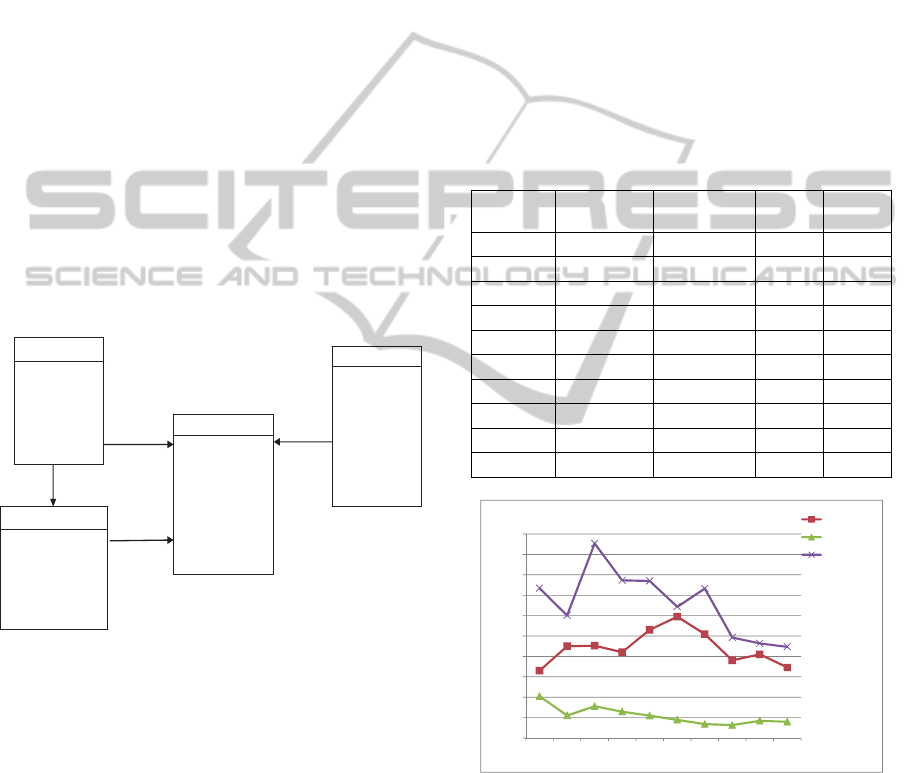
month from 150 outlets. The data warehouse is
structured as a star schema shown in Figure 4, with
the fact table (itemscan) consisting of over 21
million rows and three dimension tables viz.
storeInfo, itemDesc and storeMemberVisits.
In Section 3, the concept of inverse random
sampling without replacement (Chaudhuri and
Mukerjee, 1985); (Sangngam and Suwatee, 2010)
along with unbiased estimation techniques was
introduced for estimating the mean, Sum and M, the
count of records satisfying a property P in the
database. Next, the results of the experiments are
shown using the k-MDI tree to facilitate random
retrieval of records to estimate M.
We considered a set of three queries (modified
version of TPC-H Query 1 (TPC-H 2007) containing
the SQL functions – avg(), sum(), count() with
varying database relevancy ratios (or DRR, as
defined in Section 2.4), viz. low (<0.01), medium
(0.01 - 0.1) and high (>0.1) DRRs. The queries were
of the form:
Figure 4: The schema for experimental retail sales data
warehouse.
Select Avg(totscanAmt), Sum(totscanAmt),
Count(*)
From itemscan, storeinfo, itemdesc
Where storeno between s1 and s2
And
itemscan.storeno=storeinfo.storeno
And itemscan.itemno=itemdesc.itemno
And datesold between d1 and d2
And itemno between i1 and i2;
Table 2 shows the percentage error rates for low
database relevancy ratio, using the 10 different
sampling rates pertaining to 5 percentile values of
ρ(Q) at the 0.10 rate and 5 for 0.20 rate as per the
sampling and estimation schemes discussed in
Section 3. Here, m
1,1
refers to 0.10 rate for the 10
th
percentile value of ρ(Q); m
1,2
for the 25
th
percentile
value; m
1,3
for the 50
th
; m1,4 for 75
th
; and m
1,5
for
90
th
; while m
2,1
-m
2,5
for the same percentile values
respectively but at 0.20 rate. Table 2 and the
corresponding graph in Figure 5 show the accuracy
levels achieved by the sampling scheme using
inverse SRSWOR for low DRR queries. It is
observed that the error rates for calculation of Avg
are below 5%, but estimates of both the M and the
Sum are not within the acceptable error limits of 5%.
Table 2: Estimating for M, Avg and Sum using inverse
SRSWOR
- Low DRR
Sampling
Rate
Est. value of
M
Error in
estimating M
Error
Avg
Error
Sum
m1,1 3231 6.61 4.1 14.68
m1,2 2758 9.01 2.21 12.02
m1,3 2757 9.05 3.12 19.08
m1,4 3286 8.42 2.59 15.46
m1,5 3353 10.61 2.19 15.4
m2,1 2670 11.9 1.78 12.87
m2,2 3340 10.18 1.36 14.65
m2,3 3262 7.62 1.27 9.86
m2,4 2782 8.21 1.69 9.28
m2,5 3241 6.92 1.59 8.94
Figure 5: Error rates of estimating M, Avg and Sum using
SRSWOR for low DRR.
Table 3 and the corresponding graph in Figure 6
show the accuracy levels achieved by the sampling
scheme as described for inverse SRSWOR on
medium DRR queries. It can be observed that for
medium DRR queries, the count M, the Avg and the
Sum are within the acceptable error rate limits of 0-
5%.
ITEMSCAN
storeno
datesold
itemno
visitno
qty
totalScanAmt
unitcost
unitprice
21,421,663
ITEMDESC
itemno
categoryno
subcategoryno
primarydesc
secondarydesc
colour
sizedesc
statuscode
:
19,825
STOREINFO
storeno
storename
regionno
districtno
storetype
address
:
150
STOREMEMBERVISTS
memberno
visitno
storeno
memberstatuscode
:
218,872
0
2
4
6
8
10
12
14
16
18
20
m1,1 m1,2 m1,3 m1,4 m1,5 m2,1 m2,2 m2,3 m2,4 m2,5
Errorrate(%)
Samplingrate
EstimatingM,Avg()&Sum()‐ LowDRR
Errest.M
ErrorAvg
ErrorSum
SelectingAdequateSamplesforApproximateDecisionSupportQueries
53
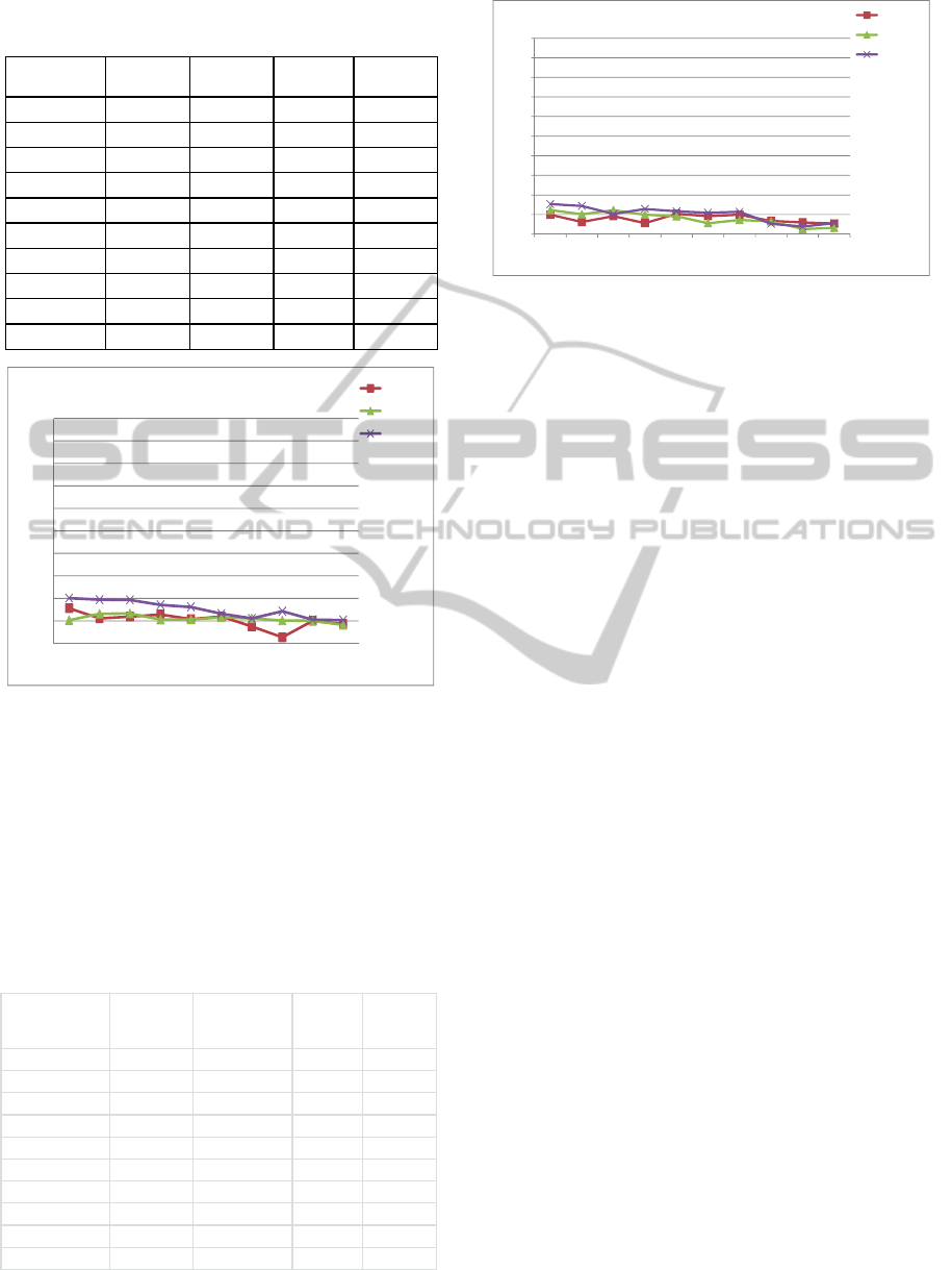
Table 3: Estimating for M, Avg and Sum using inverse
SRSWOR - Medium DRR.
Figure 6: Error rates of estimating M, Avg and Sum using
SRSWOR for medium DRR.
Table 4 and the corresponding graph in Figure 7
show the accuracy levels achieved by the sampling
scheme for inverse SRSWOR on high DRR queries.
It can be observed that the count M, the Avg and the
Sum were quite accurately estimated as they are
within the acceptable error rate limits of 0-5%.
Table 4: Estimating for M, Avg and Sum using inverse
SRSWOR - High DRR
Figure 7: Error rates of estimating M, Avg and Sum using
SRSWOR for high DRR.
In general, the accuracies achieved for high DRR
queries are better than those of medium DRR. Thus,
the sensitivities of the error rates for all the three
statistics viz., AVG, SUM and M are much less, i.e.
show fewer fluctuations, as compared to that of the
medium DRR.
5 CONCLUSIONS
In this paper, an innovative estimation scheme based
on inverse simple random sampling without
replacement (SRSWOR) was presented for
approximate processing of data warehouse queries.
Using this technique, the total number M of records
in the whole database satisfying the query conditions
was estimated along with the mean and sum for
typical queries. The k-MDI tree index was used to
draw the samples efficiently. It was found that for
queries of low database relevancy ratio (DRR), the
estimated values of average were within the
acceptable error limit of 5%, but not the estimates of
sum and the total number of relevant records M.
However, for both medium and high DRR queries,
all the three statistics viz. the value of M, the
average and the sum were estimated with error rates
below 5% as shown in Section 4. Future research
may incorporate the probabilistic approaches such as
those in (Aouiche and Lemire 2007); (Heule et al.,
2013) in our algorithm based on k-MDI tree.
REFERENCES
Aouiche, K. and Lemire, D. 2007. A Comparison of Five
Probabilistic View-Size Estimation Techniques in
OLAP, DOLAP’07, November 2007, Lisboa, Portugal.
Bentley, J. L. 1975. Multidimensional binary search trees
used for associative searching, Communications of the
Sampling
Rate
Est.ofMErrest.MErrorAvg ErrorSum
m1,1
11683 3.12
2.06 4.02
m1,2
11582 2.22
2.63 3.88
m1,3
11600 2.38
2.66 3.86
m1,4
11621 2.57
2.11 3.42
m1,5
11575 2.16
2.13 3.24
m2,1
11602 2.4
2.31 2.64
m2,2
11500 1.5
2.22 2.22
m2,3
11391 0.54
2.03 2.86
m2,4
11558 2.01
2.01 2.1
m2,5
11526 1.73
1.64 2.08
0
2
4
6
8
10
12
14
16
18
20
m1,1 m1,2 m1,3 m1,4 m1,5 m2,1 m2,2 m2,3 m2,4 m2,5
Errorrate(%)
Samplingrate
EstimatingM,Avg()&Sum()‐ MediumDRR
Errest.M
ErrorAvg
ErrorSum
SamplingRate Est.ofMErrest.MErrorAvg ErrorSum
m1,1 329333 1.97 2.45 3.06
m1,2 331819 1.23 2.01 2.87
m1,3 342099 1.83 2.44 2.05
m1,4 339680 1.11 1.98 2.56
m1,5 328997 2.07 1.82 2.32
m2,1 329803 1.83 1.1 2.18
m2,2 329299 1.98 1.44 2.28
m2,3 331449 1.34 1.29 1.05
m2,4 339949 1.19 0.52 0.76
m2,5 339546 1.07 0.63 1.11
0
2
4
6
8
10
12
14
16
18
20
m1,1 m1,2 m1,3 m1,4 m1,5 m2,1 m2,2 m2,3 m2,4 m2,5
Errorrate(%)
Samplingrate
EstimatingM,Avg()&Sum()‐ HighDRR
Errest.M
ErrorAvg
ErrorSum
ICEIS2013-15thInternationalConferenceonEnterpriseInformationSystems
54

ACM, September 1975, 18(9): 509-517.
Berenson, M. L., and D. M. Levine. 1992. Basic Business
Statistics - Concepts and Applications. Prentice Hall,
Upper Saddle River, New Jersey, USA.
Chaudhuri, A., and R. Mukerjee. 1985. Domain
Estimation in Finite Populations. Australian Journal of
Statistics. 27(2): 135-137.
Chaudhuri, S. 2012. What Next? A Half-Dozen Data
Management Research Goals for BigData and the
Cloud. PODS 2012. May 21-23. Scottsdale, Arizona,
USA.
Fisher, D. 2011. Incremental, Approximate Database
Queries and Uncertainty for Exploratory Visualization.
IEEE Symposium on Large Data Analsis and
Visualization. 73-80. October 23-24. Providence, RI,
USA.
Fisher, D., I. Popov, S. M. Drucker, and M. Schraefel.
2012. Trust Me, I’m Partially Right: Incremental
Visualization Lets Analysts Explore Large Datasets
Faster. CHI 2012, May 5-10. Austin, Texas, USA.
1673-1682.
Heule, S., Numkesser, M. and Hall, A. 2013.
HyperLogLog in Practice: Algorithmic Engineering of
a State of The Art Cardinality Estimation Algorithm.
EDBT/ICDT’13 2013, March 18-22. Genoa, Italy.
Hobbs, L., S. Hillson, and S. Lawande. 2003. Oracle9iR2
Data Warehousing. Elsevier Science, MA, USA.
Jermaine, C., 2007. Random Shuffling of Large Database
Tables. IEEE Transactions on Knowledge and Data
Engineering. 18(1):73-84.
Jermaine, C. 2003. Robust Estimation with Sampling and
Approximate Pre-Aggregation. VLDB Conference
Proceedings 2003, 886-897.
Jermaine, C., A. Pol, and S. Arumugam. 2004. Online
Maintenance of Very Large Random Samples.
SIGMOD Conference Proceedings 2004.
Jin, R., L. Glimcher, C. Jermaine, and G. Agrawal. 2006.
New Sampling-Based Estimators for OLAP Queries.
Proceedings of the 22nd International Conference on
Data Engineering (ICDE'06), Atlanta, GA, USA.
Joshi, S., and C. Jermaine. 2008. Matirialized Sample
Views for Database Approximation, IEEE
Transcaions on Knowledge and Data Engineering,
20:3 pp. 337-351.
Li, X., J. Han, Z. Yin, J-G. Lee, and Y. Sun. 2008.
Sampling Cube: A Framework for Statistical OLAP
over Sampling Data. Proceedings of ACM SIGMOD
International Conference on Management of Data
(SIGMOD'08), Vancouver, BC, Canada, June.
Olken, F., and D. Rotem. 1990. Random Sampling from
Database File. In: A Survey. International Conference
on Scientific and Statistical Database Management,
1990. pp. 92-111.
Rudra, A., R. Gopalan and N.R. Achuthan. 2012. Efficient
Sampling Techniques in Approximate Decision
Support Query Processing. Proceedings of the
International Conference on Enterprise Information
Systems - ICEIS 2012, Wroclaw, Poland. June 28-July
2 2012.
Sangngam, P., and P. Suwatee. 2010. Modified Sampling
Scheme in Inverse Sampling without Replacement.
2010 International Conference on Networking and
Information Technology. IEEE Press, New York,
USA. 580-584.
Spiegel, J., and N. Polyzotis. 2009. TuG Synopses for
Approximate Query Answering. ACM Transactions on
Database Systems. (TODS) 34(1).
TUN. 2007. Teradata University Network.
http://www.teradata.com/TUN_databases. (accessed
June 12, 2007).
TPC-H. 2007. Transaction Processing Council. Decision
Support Queries. http://www.teradata.com/
TUN_databases. (accessed April 23, 2007).
SelectingAdequateSamplesforApproximateDecisionSupportQueries
55
