A Decision-Guided Energy Framework for Optimal Power, Heating,

and Cooling Capacity Investment

Chun-Kit Ngan

, Alexander Brodsky

, Nathan Egge

and Erik Backus

Department of Computer Science, George Mason University, 4400 University Drive, Fairfax, VA 22030, U.S.A.

Facilities Management Department, George Mason University, 4400 University Drive, Fairfax, VA 22030, U.S.A.

Keywords: Decision Guidance, Energy Investment, Optimization Model.

Abstract: We propose a Decision-Guided Energy Investment (DGEI) Framework to optimize power, heating, and

cooling capacity. The DGEI framework is designed to support energy managers to (1) use the analytical and

graphical methodology to determine the best investment option that satisfies the designed evaluation

parameters, such as return on investment (ROI) and greenhouse gas (GHG) emissions; (2) develop a DGEI

optimization model to solve energy investment problems that the operating expenses are minimal in each

considered investment option; (3) implement the DGEI optimization model using the IBM Optimization

Programming Language (OPL) with historical and projected energy demand data, i.e., electricity, heating,

and cooling, to solve energy investment optimization problems; and (4) conduct an experimental case study

for a university campus microgrid and utilize the DGEI optimization model and its OPL implementations,

as well as the analytical and graphical methodology to make an investment decision and to measure trade-

offs among cost savings, investment costs, maintenance expenditures, replacement charges, operating

expenses, GHG emissions, and ROI for all the considered options.

1 INTRODUCTION

Sustainable enterprise development has been

considered a significant and competitive strategy of

corporate growth in manufacturing and service

organizations. A significant part of sustainable

development involves new technologies for local

electricity, heating, and cooling generation. Making

optimal decisions on planning and investment of

these technologies to support commercial and

industrial facilities is an involved problem because

of complex operational dependencies of these

technologies. This is exactly the focus of this paper.

Currently, the existing approaches to support the

optimization of energy plants can be divided into

two categories: (1) optimal operation of an energy

system and (2) a better plant-process design

(Broccard et al., 2010). The former category is

related to the optimized scheduling of an electric

power plant. Some researchers, such as Bojic and

Stojanovic (Bojić and Stojanović, 1998), proposed

an optimization procedure based on a MILP solver

(SAS Institute, 2012) to provide an operation

diagram which allows users to find an optimum

composition of energy consumption that minimizes

the operating expenses of an energy system

(Brodsky and Wang, 2008); (Brodsky et al., 2009);

(Brodsky et al., 2011). The latter approach includes

the analysis of simulations carried out to determine

the most suitable matching between a plant and its

loads that could increase the plant power output.

Some researchers, e.g., Savola et al., (Savola and

Keppo, 1997) did extensive research to propose an

off-design simulation and mathematical modelling

of the operation at part loads and a Mixed-Integer

Non-Linear Programming (MINLP) optimization

model for increasing power production (Savola and

Fogelholm, 2007); (Tuula Savola et al., 2007).

However, neither of the above approaches

considers optimizing the complex interactions

between the existing components and the newly

added energy equipment that would result in a

higher operating cost, such as the charges on

electricity and gas consumptions, as well as

significant environmental impacts, i.e., greenhouse

gas (GHG) emissions, e.g., carbon dioxide (CO

)

and mono-nitrogen oxide (NO

). Without

considering such interactions for every time interval

over an investment time horizon, it would be

impossible to make optimal recommendations on

357

Ngan C., Brodsky A., Egge N. and Backus E..

A Decision-Guided Energy Framework for Optimal Power, Heating, and Cooling Capacity Investment.

DOI: 10.5220/0004447503570369

In Proceedings of the 15th International Conference on Enterprise Information Systems (ICEIS-2013), pages 357-369

ISBN: 978-989-8565-59-4

 2013 SCITEPRESS (Science and Technology Publications, Lda.)

energy planning and investment.

Thus this paper focuses on addressing the above

shortcomings. More specifically, the contributions of

this paper are as follows. First, we propose a

Decision-Guided Energy Investment (DGEI)

Framework shown in Figure 1. Given electricity,

heating, and cooling generation processes, utility

contracts, historical and projected demand, facility

expansions, and Quality of Service (QoS)

requirements, the DGEI framework is designed to

recommend optimal settings of decision control

variables. These decision control variables include

the amount of electricity, heating, and cooling that is

generated by the supply of water and gas, which is

inputted to each deployed component in every time

interval. The goal of the DGEI framework is to learn

optimal values of those decision control variables in

order to minimize the total operating cost within the

required quality of service and within the bound for

GHG emissions, as well as to take into account all

components’ interactions. Second, to support the

DGEI framework, we develop a DGEI optimization

model, i.e., a MILP formulation construct, to solve

the adjusted cost minimization problem.

Furthermore, we implement the DGEI optimization

model by using the IBM Optimization Programming

Language (OPL) (Hentenryck, 1999); (The IBM

Corporation, 2012). Third, we propose an analytical

and graphical methodology to determine the best

available investment option based upon the

evaluation parameters shown in Figure 1. The

parameters include investment costs, maintenance

expenditures, replacement charges, operating

expenses, cost savings, return on investment (ROI),

and GHG emissions. Finally, we use the

methodology and the DGEI framework to conduct

an experimental case study on the microgrid at the

Fairfax campus of George Mason University

(GMU). This study has been conducted and used by

the GMU Facilities Management Department (FMD)

to make actual investment decisions.

Figure 1: Decision-Guided Energy Investment (DGEI)

Framework.

The rest of the paper is organized as follows.

Using the GMU Fairfax campus microgrid as an

example, we describe its energy investment problem

in Section 2. We explain our DGEI framework and

optimization model in Section 3 and demonstrate the

OPL implementation in Section 4. In Section 5, we

present the analytical and graphical methodology to

determine an optimal investment option. In Section

6, we conduct the experimental analysis on the

GMU energy investment case and illustrate the

relationships among the investment costs, ROI, and

GHG emissions of the various options in tabular and

graphical formats. We also explain and draw the

conclusion for the investment options from the

graphs and tables in detail on the GMU energy

investment problem. In Section 7, we conclude and

briefly outline the future work.

2 PROBLEM DESCRIPTION

OF REAL CASE STUDY

Consider the real case study at GMU, in which the

GMU Facilities Management Department (FMD) is

planning to extend and or expand the existing energy

equipment in order to meet the current and future

demand of electricity, heating, and cooling across

the expanding Fairfax campus in Virginia. Presently,

the GMU existing energy facilities at the Fairfax

campus operate a centralized heating and cooling

plant (CHCP) system and utilize the electricity

purchased from the Dominion Virginia Power

Company (DVPC) to satisfy all the energy demand.

Over the past 10 years, the campus has experienced

a significant growth on a square-foot basis in terms

of land use. Since the campus continues its

expansion at a rapid rate, the existing CHCP system

and the electricity consumption have reached a

saturated point where the current capacity and

facilities will not be able to satisfy the future energy

demand, i.e., electricity, heating, and cooling. For

these reasons, a study has been conducted to

determine the best available investment option, e.g.,

a new cogeneration (CoGen) plant, with regards to a

possible methodology to meet the current and future

electricity, heating, and cooling demand, while also

addressing the optimal operations of the newly

added facility with the existing energy equipment.

The diagram in Figure 2 depicts the GMU energy

generation process which supplies heating, cooling,

and electricity to the entire Fairfax campus. The

GMU energy facilities have a CHCP system to

supply the hot and cold water (see the red and blue

ICEIS2013-15thInternationalConferenceonEnterpriseInformationSystems

358

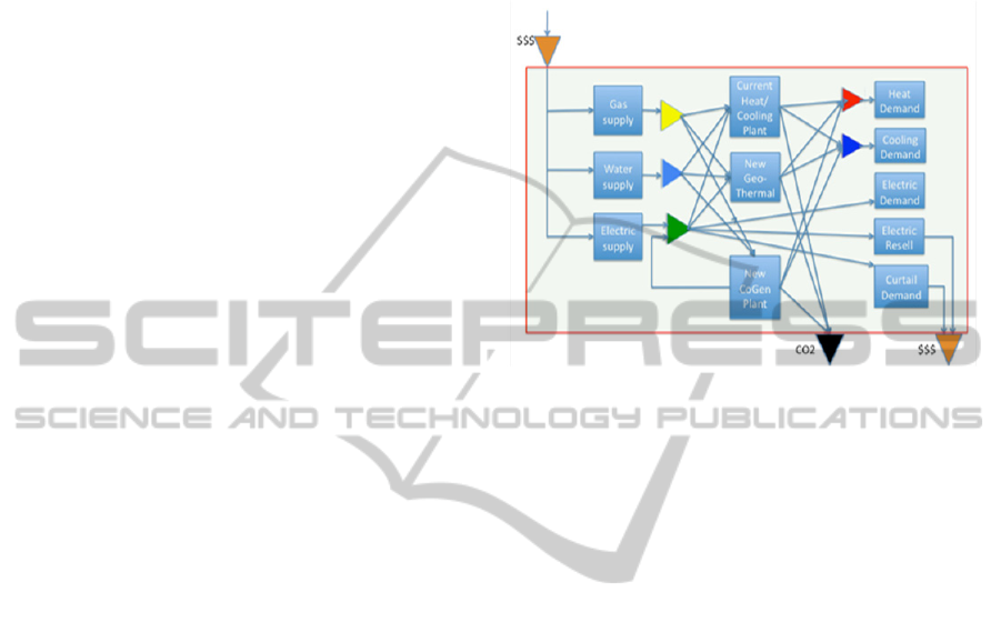
resources) which are distributed across the facilities

to the campus buildings to meet the heating and

cooling demand (see the upper two sub-processes on

the right), i.e., heating and air-conditioning to the

buildings. To supply the heating and cooling to the

campus buildings, the CHCP system needs the

inputs, i.e., natural gas (see the yellow resource on

the left), water (see the light blue resource on the

left), and electric power (see the green resource on

the left). These resources come from the gas supply,

i.e., Washington Gas Light Company (WGLC), the

water supply, i.e., Fairfax County Water Authority

(FCWA), and the electricity supply, i.e., Dominion

Virginia Power Company (DVPC), correspondingly.

In addition, the facilities also need to satisfy the

electricity demand across the entire campus, where

the electricity demand is beyond the demand from

the CHCP consumption. Any excessive electric

power supply can also be resold to the DVPC (see

the electricity resell on the right). Furthermore, the

facilities also commit a curtailment demand (see the

curtailment demand on the right) to the energy

curtailment program through EnergyConnect (EC),

Inc. Both the electricity resell and the curtailment

commitment can bring certain revenues and savings

to offset the overall operational costs on a monthly

basis and the capital expenditures in the long run.

The facilities also generate greenhouse gas (GHG)

emissions, such as carbon dioxide (CO

) (see the

black resource at the bottom right).

Given the expansion of the GMU Fairfax

campus, in addition to the increasing electricity

demand, the heating and cooling demand is also

expected to increase. The CHCP system will not

have enough capacity to meet the future need. The

GMU plan is to employ a procurement strategy, i.e.,

the deployment of the best available investment

option, which will satisfy projected demand and

minimize investment costs, maintenance

expenditures, replacement charges, operating

expenses, and GHG emissions, as well as maximize

cost savings and return on investment (ROI) at the

same time. The FMD managers are now considering

some viable options. One of the considerable options

is to integrate a new cogeneration (CoGen) plant

(see the lower sub-process in the middle), i.e., the

Combined Heating and Power (CHP) Plant (Biezma

and San Cristobal, 2006); (Broccard, et al., 2010),

into the existing facilities shown in Figure 2. The

new CoGen plant has turbines to generate electricity

to complement the electricity demand, uses the

generated heat as a by-product to complement the

heating demand, and collaborates with the ammonia

process technology (American Electric Power Inc.,

2012) to supply the cooling demand. Now, the

challenging question is how to analytically

determine the best investment option that satisfies all

the energy demand, i.e., electricity, heating, and

cooling, at the lowest operating costs.

Figure 2: Prospective Heating, Cooling, and Electric

Power Facilities at the GMU Fairfax campus.

3 DECISION-GUIDED ENERGY

INVESTMENT (DGEI)

FRAMEWORK

AND OPTIMIZATION MODEL

To answer the above question, we propose the DGEI

framework depicted in Figure 1. This framework is

composed of six energy-investment libraries, i.e.,

Energy Generation Process (EGP), Energy

Contractual Utility (ECU), Energy Historical

Demand (EHD), Energy Future Demand (EFD),

Energy Facility Expansion (EFE), Quality of Service

(QoS) requirements, and a DGEI optimizer. The

EGP is an extensible library that enables domain

experts to construct an energy generation process to

supply electricity, heating, and cooling. The ECU is

a library that contains energy contractual terms for

calculating bill utilities, e.g., an electricity bill, a

water bill, and a gas bill. The EHD and EFD are the

libraries that store historical and projected energy

demand respectively. The EFE library archives the

facility expansion of an organization in terms of

square-footage increase. The QoS library stores the

QoS requirements that the energy facilities of an

organization need to meet, e.g., the maximal power

interruptions allowed per monthly pay period in an

organization. The DGEI optimizer supports energy

managers to utilize all the libraries, i.e., EGP, ECU,

EHD, EFD, EFE, and QoS, as inputs to the decision

ADecision-GuidedEnergyFrameworkforOptimalPower,Heating,andCoolingCapacityInvestment

359

optimization process, which minimizes operating

expenses and maximize cost savings. This decision

optimization process not only optimizes the

interactions between the existing and the

considerable energy facility options but also

minimizes the environmental impacts on the

surroundings, i.e., minimizing the GHG emissions.

In addition to the GHG emissions, energy managers

also utilize (1) return on investment (ROI), i.e., the

gain return efficiency among different investments,

(2) the investment costs, i.e., an amount spent to

acquire a long-term asset, and (3) equipment

expenses, i.e., maintenance expenditures plus

replacement charges, to evaluate all the available

investments and then to determine the best option.

To solve an energy investment optimization

problem in terms of minimizing the operating cost

and the GHG emissions is to formulate a DGEI

optimization model. This model optimally learns

decision control variables, which require several

input data sets, i.e., the historical and projected

electricity, heating, and cooling demand over a time

horizon, the electric and gas contractual utility, the

operational parameters and capacity constraints of

the existing and the new electric power plants, as

well as the energy aggregation of the supply and

demand, e.g., electricity, gas, heating, and cooling,

to minimize the entire operating expenses. Using the

GMU energy investment optimization problem over

the 10-year time horizon as an example, we explain

the above terminologies used in this case study in

the following subsections.

3.1 Electricity, Heating, and Cooling

Demand over a Time Horizon

The electricity, heating, and cooling demand over a

time horizon is the input, including the usage of the

historical and projected quantities, which are

provided from the GMU Facilities Management

Department, to the DGEI optimization model that

requires the domain users to define all (i.e., past plus

future), past, and future power intervals over the 10-

year time horizon.

 AllPowerIntervals is a set of all powerIntervals,

where each powerInterval is a tuple which includes

several attributes, i.e., pInterval, payPeriod, year,

month, day, hour, and weekDay. We use negative

and zero integers to represent the past time horizon

and positive integers to denote the future time

horizon. For example, pInterval is an hourly time

interval of the energy demand, where -8759 ≤

pInterval ≤ 78840. payPeriod is a monthly pay

period of the energy demand, where -11 ≤

payPeriod ≤ 108. Other attributes’ intervals

include 2011 ≤ year ≤ 2020, 1 ≤ month ≤ 12, 1 ≤

day ≤ 31, 0 ≤ hour ≤ 23, and 0 ≤ weekDay ≤ 6.

 PastPowerIntervals is a set of past powerIntervals

of tuples, where -8759 ≤ pInterval ≤ 0, -11 ≤

payPeriod ≤ 0, year = 2011, 1 ≤ month ≤ 12, 1 ≤

day ≤ 31, 0 ≤ hour ≤ 23, and 0 ≤ weekDay ≤ 6.

 FuturePowerIntervals is a set of future

powerIntervals of tuples, where 1 ≤ pInterval ≤

78840, 1 ≤ payPeriod ≤ 108, 2012 ≤ year ≤ 2020, 1

≤ month ≤ 12, 1 ≤ day ≤

31, 0 ≤ hour ≤ 23, and 0 ≤

weekDay ≤ 6.

After declaring the power intervals, the quantities

of electricity, heating, and cooling demand can be

stored in their arrays over their power intervals.

These three quantities of demand are provided by

the GMU Facilities Management Department.

 demandKw[AllPowerIntervals] ≥ 0 is an array of

electricity demand over the AllPowerIntervals.

This array stores both the historical and the

projected demand over the PastPowerIntervals and

the FuturePowerIntervals respectively.

 demandHeat[FuturePowerIntervals] ≥ 0 is an array

of projected heating demand over the

FuturePowerIntervals.

 demandCool[FuturePowerIntervals] ≥ 0 is an array

of projected cooling demand over the

FuturePowerIntervals.

3.2 Electric and Gas Contractual

Utility

To determine the total operating cost, we need to

compute the consumption expenses of electricity and

gas supply according to their utility contracts.

The consumption expenses of electricity include

both the peak demand charge and the total power

consumption charge that are explained in detail as

follows.

3.2.1 Peak Demand Charge

For the electricity supply,

utilityKw[AllPowerIntervals] ≥ 0 is an array of

electricity supplied from the DVPC over the

AllPowerIntervals.

historicUtilityKw[i] is an array of past electricity

demand from the GMU, i.e.,

historicUtilityKw[i] = demandKw[i],

which satisfies the constraint, i.e., utilityKw[i]

== historicUtilityKw[i], where i ∈

PastPowerIntervals. This constraint is to assure that

the electricity consumed by the GMU in the past

ICEIS2013-15thInternationalConferenceonEnterpriseInformationSystems

360

year, i.e., 2011, is equivalent to the supply from the

DVPC.

payPeriodSupplyDemand[p] is the peak demand

usage per future pay period (p). This peak demand

usage meets the below contractual constraints (C1

and C2) and is determined based upon the highest of

either (C1) or (C2):

C1: The highest average kilowatt measured in

any hourly time interval of the current billing month

during the on-peak hours of either between 10 a.m.

and 10 p.m. from Monday to Friday for the billing

months of June through September or between 7

a.m. and 10 p.m. from Monday to Friday for all

other billing months.

C2: 90% of the highest kilowatt of demand at the

same location as determined under (C1) above

during the billing months of June through September

of the preceding eleven billing months.

The logic constraints of both C1 and C2 can be

expressed as follows:

if (i.payPeriod == p ∧ i.weekDay ≥ 1

∧ i.weekDay ≤ 5 ∧ ((i.month ≥ 6 ∧

i.month ≤ 9 ∧ i.hour ≥ 10 ∧ i.hour ≤

22) ∨ (i.month ≤ 5 ∧ i.month ≥ 10 ∧

i.hour ≥ 7 ∧ i.hour ≤ 22)))

payPeriodSupplyDemand[p] ≥

utilitykW[i]

else if (i.month ≥ 6 ∧ i.month ≤ 9 ∧

i.payPeriod ≥ p – 11 ∧ i.payPeriod ≤ p

∧ i.weekPay ≥ 1∧ i.weekDay ≤ 5 ∧ i.hour

≥ 10 ∧ i.hour ≤ 22)

payPeriodSupplyDemand[p] ≥ 0.9 *

utilitykW[i];

, where i ∈

AllPowerIntervals, p ∈ FuturePayPeriods, and 1 ≤

FuturePayPeriods ≤ 108. Using these logic

constraints, we can determine the optimal peak

demand usage per future pay period, which

consumes more than the expected electricity supply

per powerInterval from the DVPC.

generationDemandCharge[p], i.e.,

generationDemandCharge[p] = 8.124 *

payPeriodSupplyDemand[p];, is the Electricity

Supply (ES) service charge, i.e., the peak demand

charge, where p ∈ FuturePayPeriods, and 8.124 is

the dollar charge per kW.

3.2.2 Total Power Consumption Charge

payPeriodKwh[p] is the total power consumption

per future pay period, i.e.,

payPeriodKwh[p] =

∑utilitykW[i];, where i ∈ AllPowerIntervals, p

∈ FuturePayPeriods, and i.payPeriod = p.

payPeriodKwhCharge[p] is the total kWh charge

per future pay period, i.e., payPeriodKwhCharge[p]

≥ 0, which satisfies the below contractual

constraints:

if (payPeriodKwh[p] ≤ 24000)

payPeriodKwhCharge[p] = 0.01174 *

payPeriodKwh[p]

else if (payPeriodKwh[p] ≤ 210000)

payPeriodKwhCharge[p] = 0.01174 *

24000 + 0.00606 *

(payPeriodKwh[p] – 24000)

else

payPeriodKwhCharge[p] = 0.01174 *

24000 + 0.00606 * 186000 +

0.00244 * (payPeriodKwh[p] –

210000);

, where p ∈ FuturePayPeriods,

0.01174 is the dollar charge of the first 24000 kWh

consumed, 0.00606 is the dollar charge of the next

186000 kWh consumed, and 0.00244 is the dollar

charge of the additional kWh consumed. Note that if

payPeriodSupplyDemand[p] is 1000 kW or more,

210 kWh for each peak demand usage over 1000 kW

is added to the total power consumption to calculate

payPeriodKwhCharge[p].

3.2.3 Total Electricity Cost

The total electricity cost per future pay period is the

sum of payPeriodKwhCharge[p] and

generationDemandCharge[p], i.e.,

electricCostPerFuturePayPeriod =

(payPeriodKwhCharge[p] +

generationDemandCharge[p]);

, where p ∈

FuturePayPeriods.

Table 1: Descriptions for the Constant Values in the DGEI

Optimization Model of the GMU Energy Investment

Problem.

Constant Description

0.9

Percentage of the highest kW of demand

during the billing months of June through

September of the preceding 11 billing

months

8.124

Amount ($) of Electricity Supply (ES)

demand charged per kW

24000 First ES kWh

0.01174

Amount ($) of the first 24000 ES kWh

charged per kWh

186000 Next ES kWh

0.00606

Amount ($) of the next 186000 ES kWh

charged per kWh

210000

Sum of the first ES kWh and the next ES

kWh

0.00244

Amount ($) of the additional ES kWh

charged per kWh

210

kWh for each ES kW of demand over 1000

The total electricity cost of all the

ADecision-GuidedEnergyFrameworkforOptimalPower,Heating,andCoolingCapacityInvestment

361

FuturePayPeriods is the aggregations of all the total

electricity costs per future pay period, i.e.,

electricCost = ∑(payPeriodKwhCharge[p]

+ generationDemandCharge[p]);, where p ∈

FuturePayPeriods.

Table 1 summarizes the descriptions of all the

constant values from the electric utility contract used

in the DGEI optimization model for the GMU

energy investment problem.

3.2.4 Total Gas Consumption Charge

Regarding the gas supply,

utilityGas[FuturePowerIntervals] ≥ 0 is an array of

gas supplied from the WGLC over the

FuturePowerIntervals. The total gas cost of all the

FuturePowerIntervals is the aggregations of all the

total gas utility per future power interval, i.e.,

gasCost = (∑(utilityGas[i]/btuPerDth))

* gasPricePerDth;, where i ∈

FuturePowerIntervals, btuPerDth = 1000000 BTU,

which is the amount of energy per decatherm, and

gasPricePerDth = $6.5, which is the gas charge per

decatherm.

3.2.5 Total Operating Cost

The total operating cost is the sum of the total

electricity cost of all the future pay periods and the

total gas cost of all the future power intervals, i.e.,

totalCost = electricCost + gasCost;.

3.3 Operational Parameters

and Capacity Constraints

of the CHCP and the Cogen Plant

In addition to the supply and demand of gas and

electricity, the operational parameters and the

capacity constraints of the CHCP and the CoGen

plant are also considered.

3.3.1 The CHCP Plant

For the CHCP plant,

gasIntoCHCP[FuturePowerIntervals] ≥ 0 is an array

of natural gas input to the CHCP over the

FuturePowerIntervals to generate the heat supply.

kwIntoCHCP[FuturePowerIntervals] ≥ 0 is an array

of power input to the CHCP over the

FuturePowerIntervals to generate the cool supply.

heatOutCHCP[FuturePowerIntervals] ≥ 0 is an array

of heat output from the CHCP over the

FuturePowerIntervals to satisfy the partial heating

demand. coolOutCHCP[FuturePowerIntervals] ≥ 0

is an array of cool output from the CHCP over the

FuturePowerIntervals to satisfy the partial cooling

demand. The CHCP constraints include:



heatOutCHCP[i] * gasPerHeatUnit ≤

gasIntoCHCP[i];, i.e., the amount of gas

consumed to generate the heat cannot be more than

that of the gas input;



coolOutCHCP[i] * kwhPerCoolUnit ≤

kwIntoCHCP[i];, i.e., the amount of electric

power consumed to generate the cool cannot be

more than that of the power input;



heatOutCHCP[i] ≤ chcpMaxHeatPerHr;, i.e.,

the amount of heat generated cannot be more than

the maximal heat output of the CHCP; and



coolOutCHCP[i] ≤ chcpMaxCoolPerHr;, i.e.,

the amount of cool generated cannot be more than

the maximal cool output of the CHCP, where i ∈

FuturePowerIntervals, gasPerHeatUnit = (1 / 0.78),

and kwhPerCoolUnit = (1 / 0.94).

3.3.2 The CoGen Plant

For the CoGen plant,

gasIntoCogen[FuturePowerIntervals] ≥ 0 is an array

of gas input to the CoGen plant over the

FuturePowerIntervals to generate the power supply.

kwOutCogen[FuturePowerIntervals] ≥ 0 is an array

of power output from the CoGen plant over the

FuturePowerIntervals to satisfy the partial electricity

demand. heatOutCogen[FuturePowerIntervals] ≥ 0 is

an array of heat output from the CoGen plant over

the FuturePowerIntervals to satisfy the partial

heating demand.

coolOutCogen[FuturePowerIntervals] ≥ 0 is an array

of cool output from the CoGen plant over the

FuturePowerIntervals to satisfy the partial cooling

demand. The constraints of the CoGen plant include:



kwOutCogen[i] * cogenGasPerKwh ≤

gasIntoCogen[i];, i.e., the amount of gas

consumed to generate the power cannot be more

than that of the gas input;



kwOutCogen[i] ≤ cogenMaxKw;, i.e., the

amount of power generated cannot be more than

the maximal electricity output of the CoGen plant;



heatOutCogen[i] ≤ cogenHeatPerKwh *

kwOutCogen[i];

, i.e., the amount of heat

generated cannot be more than the maximal heat

supply that is restricted by the power output of the

CoGen plant;



heatOutCogen[i] ≤ cogenMaxHeatPerHr *

(kwOutCogen[i]/cogenMaxKw);, i.e., the

amount of heat generated cannot be more than the

maximal heat output of the CoGen plant;



coolOutCogen[i] ≤ (cogenMaxHeatPerHr *

(kwOutCogen[i]/cogenMaxKw) -

ICEIS2013-15thInternationalConferenceonEnterpriseInformationSystems

362

heatOutCogen[i]) *

cogenHeatToCoolRatio;, i.e., the amount of

cool generated cannot be more than the maximal

cool supply that is restricted by the power and heat

output of the CoGen plant; and



coolOutCogen[i] ≤ cogenMaxCoolPerHr;,

i.e., the amount of cool generated cannot be more

than the maximal cool output of the CoGen plant,

where i ∈ FuturePowerIntervals, cogenMaxKw =

7200 kW is the maximal power output,

cogenHeatPerKwh = 10300 kWh is the amount of

heat generated per kWh, cogenHeatToCoolRatio =

cogenMaxCoolPerHr/cogenMaxHeatPerHr is the

ratio of converting heat to cool supply,

cogenMaxHeatPerHr = 40000000 BTU is the

maximal heat supply of the CoGen plant per hour,

cogenMaxCoolPerHr = 2400 Tons is the maximal

cool supply of the CoGen plant per hour,

cogenGasPerKwh =

gasBTUPerGallon/kWhPerGallon/cogenGasToKwh

Efficiency is the amount of natural gas consumed

per kWh, for gasBTUPerGallon = 114000 BTU is

the amount of energy generated per gallon of gas,

kwhPerGallon = 33.41 is the amount of kWh

generated per gallon of gas, and

cogenGasToKwhEfficiency = 0.33 is the efficiency

of the CoGen plant to generate power from natural

gas.

3.4 Energy Aggregations of Supply

and Demand

The aggregations of energy supply and demand

within the entire energy system include:



kwIntoCHCP[i] + demandKw[i] ≤

utilityKw[i] + kwOutCogen[i];, i.e., the

amount of power input to the CHCP and the power

demand from the GMU cannot exceed the amount

of power supply provided from the DVPC and the

power output generated from the CoGen plant,

where i ∈ FuturePowerIntervals.



demandReduction[i] ≤ (utilityKw[i] +

kwOutCogen[i]) - (kwIntoCHCP[i] +

demandKw[i]);

, i.e., the power supply reduction

cannot exceed the difference between the total

power supply (utilityKw[i] + kwOutCogen[i]) and

the total power demand (kwIntoCHCP[i] +

demandKw[i]), where

demandReduction[FuturePowerIntervals] ≥ 0 is an

array of extra power supply that can be cut from

the power inputs over the FuturePowerIntervals,

and i ∈ FuturePowerIntervals.



∑demandReduction[i] ≤

maxKwReductionPerPayPeriod;

, i.e., the total

power reductions over the future power intervals

cannot exceed the allowable maximal power

interruptions per future pay period, where i ∈

FuturePowerIntervals, p ∈ FuturePayPeriods, and

i.payPeriod = p.



utilityGas[i] ≥ gasIntoCogen[i] +

gasIntoCHCP[i];, i.e., the gas input to the

CoGen plant and to the CHCP cannot exceed the

gas supply provided from the WGLC, where i ∈

FuturePowerIntervals.



heatOutCogen[i] + heatOutCHCP[i] ≥

demandHeat[i];, i.e., the heat demand from

GMU cannot exceed the heat supply generated

from the CoGen plant and the CHCP, where i ∈

FuturePowerIntervals.



coolOutCogen[i] + coolOutCHCP[i] ≥

demandCool[i];, i.e., the cool demand from

GMU cannot exceed the cool supply generated

from the CoGen plant and the CHCP, where i ∈

FuturePowerIntervals.

3.5 DGEI Optimization Model

After declaring all the input data sets and the above

constraints, which the input data sets need to satisfy,

the DGEI optimization model for the GMU energy

investment problem can be formulated as follows in

Figure 3.

Figure 3: The DGEI Optimization Model for the GMU

Energy Investment Problem.

ADecision-GuidedEnergyFrameworkforOptimalPower,Heating,andCoolingCapacityInvestment

363

4 OPL IMPLEMENTATION

FOR DGEI OPTIMIZATION

MODEL

The DGEI optimization model has been

implemented by using the OPL language. Using the

GMU historical data of power usage in the past year,

i.e., 2011, and its projected electricity, cooling, and

heating demand over a future time horizon from

2012 to 2020, we use the OPL language to

implement and demonstrate the DGEI optimization

model to solve the GMU energy investment problem

and minimize the operating cost.

The intuition of using the OPL language is that

its optimization formulation looks like the DGEI

optimization model. When comparing the DGEI

optimization model in Figure. 3 with the OPL

formulation from Figure 4.1 to Figure 4.9, we realize

that both models are very similar to each other. Only

some notations and syntaxes are different that is

shown in Table 2. For example, instead of using the

summation sign (∑) in the DGEI optimization

model, the OPL language uses the keyword, “sum”,

to perform the aggregation. Rather than using the if-

then statement in the mathematics, the OPL uses the

specific construct with the implication operatior

(=>).

Table 2: Differences between DGEI Optimization model

and OPL formulation model.

DGEI Optimization Model OPL Formulation Model

Notation: Summation Sign

∑

Example:

∑(demandKw[i] – kW[i]) ≤

2 * annualBound

Syntax: sum

Example:

sum(i in PowerIntervals :

i.pInterval >= 1)

(demandKw[i] - kW[i]) <=

annualBound * 2

Notation: If-then Statement

Example:

if (payPeriodKwh[p] ≤

24000)

payPeriodKwhCharge[p] =

0.01174 * payPeriodKwh[p]

Syntax: =>

Example:

(payPeriodKwh[p] <=

24000) =>

(payPeriodKwhCharge[p]

== 0.01174 *

payPeriodKwh[p])

Notation: Where clause

Example:

peakDemandBound[p] ≤

payPeriodSupplyDemand[p

], where p ∈ PayPeriods

Syntax: forall

Example:

forall (p in PayPeriods)

peakDemandBound[p] <=

payPeriodSupplyDemand[

More specifically, the OPL implementation

construct is described as follows. In Figure 4.1, from

the line number 9 to 12, the value 12, i.e., the total

12 months of 2011, is assigned to the variable

nbPastPayPeriods, the value 108, i.e., the total 108

months from 2012 to 2020, is assigned to the

variable nbPayPeriods, and the value 0 is assigned to

the maximal power interruptions, i.e.,

maxKwReductionPerPeriod. The FuturePayPeriods

is ranged from 1 to 108. From the line number 15 to

23, we declare a tuple of a power interval that has

the attributes, including pInterval, payPeriod, year,

month, day, hour, and weekDay. The line number 25

to 27 declares and initializes AllPowerIntervals that

include both PastPowerIntervals and

FuturePowerIntervals. The line number 30 to 32

declares and initializes the

demandKw[AllPowerIntervals], the

demandHeat[FuturePowerIntervals], and the

demandCool[FuturePowerIntervals] arrays.

Figure 4.1: General and Demand Input Data.

Figure 4.2: Total Electricity Cost.

Figure 4.2 declares the decision control variables,

i.e., utilityKw[AllPowerIntervals],

payPeriodSupplyDemand[FuturePayPeriods], and

payPeriodKwh[FuturePayPeriods], to compute

payPeriodKwhCharge[FuturePayPeriods] and

ICEIS2013-15thInternationalConferenceonEnterpriseInformationSystems

364

generationDemandCharge[FuturePayPeriods] that

are summed together to determine the total

electricity cost over all the future pay periods while

satisfying the electric contractual constraints.

Figure 4.3 declares the constants, i.e.,

gasPricePerDth and btuPerDth, and

utilityGas[FuturePowerIntervals] to calculate the

total gas cost over all the future power intervals.

Figure 4.3: Total Gas Cost.

Figure 4.4 declares the objective function to

minimize the total operating cost, i.e., the total

electricity cost plus the total gas cost.

Figure 4.4: Total Operating Cost.

Figure 4.5 declares the constants, i.e.,

gasPerHeatUnit, kwhPerCoolUnit,

chcpMaxHeatPerHr, and chcpMaxCoolPerHr, and

the arrays, i.e.,

gasIntoCHCP[FuturePowerIntervals],

kwIntoCHCP[FuturePowerIntervals],

heatOutCHCP[FuturePowerIntervals], and

coolOutCHCP[FuturePowerIntervals], used in the

CHCP capacity constraints.

Figure 4.5: Operational Parameters and Data Structures of

the CHCP Plant.

Figure 4.6 declares the constants from the line

number 71 to 79, and the arrays, i.e.,

gasIntoCogen[FuturePowerIntervals],

heatOutCogen[FuturePowerIntervals],

coolOutCHCP[FuturePowerIntervals], and

kwOutCHCP[FuturePowerIntervals], which are used

in the capacity constraints of the CoGen plant.

Figure 4.6: Operational Parameters and Data Structures of

the CoGen Plant.

Figure 4.7 defines all the capacity constraints for the

CHCP and the CoGen plant.

Figure 4.7: Capacity Constraints of the CHCP and the

CoGen Plant.

Figure 4.8 defines the contractual constraints for the

electricity bill.

Figure 4.8: Contractual Electricity Utility Constraints.

ADecision-GuidedEnergyFrameworkforOptimalPower,Heating,andCoolingCapacityInvestment

365

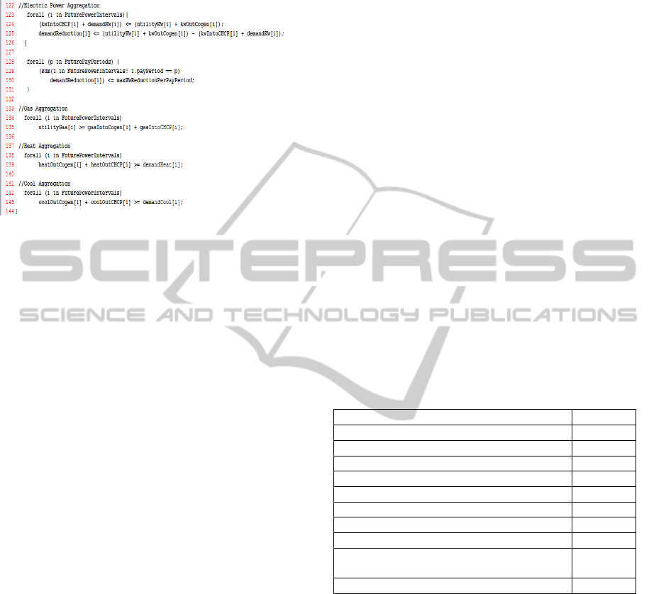
Figure 4.9 defines the constraints for the energy

aggregations of electric power, gas, heat, and cool.

Figure 4.9: Energy Aggregations of Supply and Demand.

5 ANALYTICAL

METHODOLOGY ON

EVALUATION AMONG

ENERGY INVESTMENT

OPTIONS

For domain experts being able to formulate and

implement the above DGEI optimization model to

determine the best investment option, we propose an

analytical methodology that guides the domain

experts to achieve this goal. The methodology

includes six steps.

STEP 1: Collect historical energy demand, such

as electricity, heating, and cooling, from each

building unit, and forecast those demands in terms of

growth on a square-foot basis over the future time

horizon.

STEP 2: Identify all the possible energy

investment options, such as the expansion of current

facilities and the procurement of cogeneration

plants.

STEP 3: Formulate, implement, and execute the

DGEI optimization model that integrates historical

and projected energy demand, electric and gas

contractual utility, operational parameters and

capacity constraints of energy equipment, as well as

energy aggregations of supply and demand in each

considered option under the assumption of optimal

interactions among available resources.

STEP 4: Compute the annualized evaluation

parameters for each option based upon the results

from the optimization process in STEP 3.

The parameters include the investment cost (I

equipment cost (E

), i.e., maintenance expenditure

) plus replacement charge (R

), operating expense

), i.e., the charges on electricity and gas

consumptions, cost saving (S

), i.e., C

– C

, where i

≥ 0 denotes an investment option and C

is the

operating cost of a base investment option that the

other available options compare with, and return on

investment (ROI

), i.e., S

/ (I

– I

), as well as the

GHG emissions (MTCDE

), i.e., G

* 0.053

MTCDE/Million-Btu + P

* 0.513 MTCDE/Million-

Wh, shown in Table 3, against the various

investment options, where 0.053 and 0.513 are the

factors, which are calculated from the historical data.

Note that the base investment option is the option

that the current capacity of the existing facilities is

expanded without procuring any new energy

equipment.

Using the ROI and GHG emissions, domain

users and experts can plot the analytical graphs to

illustrate the relationships among the ROI, GHG

emissions, and investment expenses, which enable

the domain experts to determine the best investment

option among all of the options being considered.

Table 3: Evaluation Parameters of ROI and GHG

Emissions for Determining the Best Investment Option.

Parameter Symbol

Investment Cost I

Maintenance Expenditure M

Replacement Charge R

Equipment Cost E

Operating Expense C

Cost Saving S

Return on Investment ROI

Average Annual Gas Consumption MBTU G

Average Annual Electric Power

Consumption MWh

GHG Emission MTCDE

STEP 5: Remove any option that is dominated by

the other options in terms of the evaluation

parameters.

STEP 6: Construct a trade-off graph to evaluate

the options that are not dominated among others and

then make a final decision.

Note that although STEP 1, 2, 4, 5, and 6 are

typical processes of evaluations, STEP 3 is not

typical at all as the problem that we solve is a non-

trivial optimization problem.

ICEIS2013-15thInternationalConferenceonEnterpriseInformationSystems

366

6 ANALYTICAL

METHODOLOGY

ON EXPERIMENTAL CASE

STUDY

After the process from STEP 1 to STEP 3 in the

experimental case study at GMU, the four

investment options, including ① the expansion of

the existing CHCP only, ② the addition of a CoGen

plant to the existing CHCP, ③ the half capacity of

the Option ① with the half planned capacity of the

CoGen plant, and ④ the full capacity of the Option

① with the full planned capacity of the CoGen

plant, have been chosen to be evaluated to meet the

electricity, heating, and cooling demand of the

Fairfax campus over the next 9 years from 2012 to

2020.

In STEP 4, using the evaluation parameters, i.e.,

ROI and GHG emissions, discussed in Section 5 and

the OPL to solve the GMU energy investment

problem in Section 4, we obtained Table 4 and

Figure 5 that can be used to determine the best

investment option.

Table 4: Evaluation Parameters of ROI and GHG

Emissions for Determining the GMU Energy Investment

Options.

Investment

Option

Investment Cost

($M)

Annual

Maintenance

Cost ($)

1 Expanded

CHCP

$34.293

$343,200

1 CoGen Plant

+ 1 Current

CHCP

$65.328 $655,600

½ CoGen Plant

+ ½ Expanded

CHCP

$46.995 $499,400

1 CoGen Plant

+ 1 Expanded

CHCP

$99.621 $998,800

Investment

Option

Annualized

Replacement

Cost ($M)

Annualized

Equipment Cost

($M)

1 Expanded

CHCP

$3.429 $3.772

1 CoGen Plant

+ 1 Current

CHCP

$3.850 $4.506

½ CoGen Plant

+ ½ Expanded

CHCP

$4.699 $5.199

1 CoGen Plant

+ 1 Expanded

CHCP

$7.279 $8.278

Table 4: Evaluation Parameters of ROI and GHG

Emissions for Determining the GMU Energy Investment

Options. (Cont.)

Investment

Option

Annualized

Average

Operational

Cost ($M)

Annualized

Saving over the

Expanded

CHCP ($M)

1 Expanded

CHCP

$6.244 $0.000

1 CoGen Plant

+ 1 Current

CHCP

$5.494 $0.016

½ CoGen Plant

+ ½ Expanded

CHCP

$5.557 -$0.740

1 CoGen Plant

+ 1 Expanded

CHCP

$5.492 -$3.754

Investment

Option

ROI (%)

Average Annual

Gas

Consumption

(MBTU)

1 Expanded

CHCP

0.000% 510,500.00

1 CoGen Plant

+ 1 Current

CHCP

0.052% 523,622.22

½ CoGen Plant

+ ½ Expanded

CHCP

-5.827% 520,888.89

1 CoGen Plant

+ 1 Expanded

CHCP

-5.747% 523,600.00

Investment

Option

Average Annual

Electric Power

Consumption

(MWh)

GHG Emission

(MTCDE)

1 Expanded

CHCP

141,433.33 99611.799

1 CoGen Plant

+ 1 Current

CHCP

141,333.33 100255.977

½ CoGen Plant

+ ½ Expanded

CHCP

141,344.44 100116.811

1 CoGen Plant

+ 1 Expanded

CHCP

141,333.33 100254.799

In STEP 5, the Option ③ and ④ are the dominated

cases that can be removed from our consideration

list because of the negative ROI.

In STEP 6, according to the Table 4 and Figure

5, we can conclude that the Option ① should be

chosen because of the three observations. First, the

GHG emissions and the equipment cost of the

Option ① are the lowest. Second, even though the

ADecision-GuidedEnergyFrameworkforOptimalPower,Heating,andCoolingCapacityInvestment

367

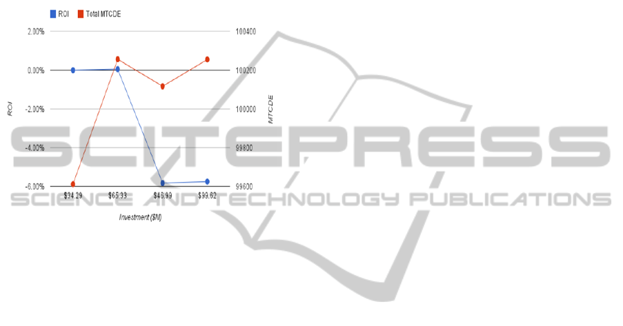
ROI of the Option ②, i.e., 0.052%, is marginally

better than that of the Option ①, the GHG

emissions of the Option ② is the highest among all

the options being considered. Third, it is not

economical at all for GMU to invest $31 million

dollars, i.e., the Option ② investment cost minus

the Option ① investment cost, more to earn only

0.052% ROI in the next 9-year timeframe. Thus, the

Option 1 is the best long-term option for GMU.

Figure 5: ROI (%) and GHG Emissions (MTCDE) vs.

Investment Cost ($M) across the Four Investment Options.

7 CONCLUSIONS AND FUTURE

WORK

In this paper, we propose a Decision-Guided Energy

Investment (DGEI) Framework to optimize power,

heating, and cooling capacity. The DGEI framework

is designed to support energy managers to (1) use

the analytical and graphical methodology to

determine the best investment option that satisfies

the designed evaluation parameters, such as ROI and

GHG emissions; (2) develop a DGEI optimization

model to solve energy investment problems that the

operating expenses are minimal in each considered

investment option; (3) implement the DGEI

optimization model using the IBM OPL language

with historical and projected energy demand data,

i.e., electricity, heating, and cooling, to solve energy

investment optimization problems; and (4) conduct

an experimental case study on the Fairfax campus

microgrid at George Mason University (GMU) and

utilize the DGEI optimization model and its OPL

implementations, as well as the graphical and

analytical methodology to make the investment

decision and trade-offs among the cost savings,

investment costs, maintenance expenditures,

replacement charges, operating expenses, GHG

emissions, and return on investment (ROI) for all the

considered options.

Technically, the core challenge is the

development of the DGEI optimization model that is

very accurate in terms of the contractual terms and

engineering constraints, and yet efficient and

scalable, which is done by the careful modelling of

mainly continuous decision variables and using

constructs that avoid introduction of combinatorics,

e.g., explicit or implicit binary variables, into the

model. However, the DGEI optimization problem

that we formulate is implemented by using the OPL

language. This OPL construct is then sent to the

IBM CPLEX solver which is the branch-and-bound-

based algorithm with the exponential time

complexity, i.e., 2



, where k is the number of

decision control variables, and N is the size of the

learning data set. Thus the furture research focus

will develop a new algorithm that will be able to

solve the energy investment problems at a lower

time complexity.

Concerning the real case study at George Mason

University and its CHCP system, it is clear that

GMU must develop and research other available

options beyond those discussed in the analysis of

this paper in order to meet the future needs of the

Fairfax campus demand. Thus, the DGEI framework

further developed will aid the GMU energy decision

makers to determine the optimal solutions that will

satisfy the GMU short- and long-term power,

heating, and cooling demand. Note that our

framework is applicable to solve any energy

investment problem in different domains of industry.

Therefore, the future work includes the advanced

development of the DGEI libraries and optimization

models that enable domain users and experts to

integrate more clean and efficient energy equipment,

such as geothermal electric power facilities, into the

existing plants optimally in order to support the

continuous development of enterprises and

organizations.

REFERENCES

Alrazgan, A., Nagarajan, A., Brodsky, A., and Egge, N.,

(2011). Learning Occupancy Prediction Models with

Decision-Guidance Query Language. Proceedings of

the 44

Hawaii International Conference on System

Sciences. Koloa, Kauai, Hawaii, U.S.A.

American Electric Power Inc., (2012). CCS Front End

Engineering & Design Report American Electric

Power Mountaineer CCS II Project Phase 1.

Columbus, Ohio, U. S. A.

http://cdn.globalccsinstitute.com/sites/default/files/pub

ICEIS2013-15thInternationalConferenceonEnterpriseInformationSystems

368

lications/32481/ccs-feed-report-gccsi-final.pdf on

January 30, 2012.

Biezma, M. and San Cristobal, J., (2006). Investment

Criteria for the Selection of Cogeneration Plants – a

State of the Art Review. Journal of Applied Thermal

Engineering, Vol. 26 Issues 05 - 06, p. 583–588.

Broccard, M., Girdinio, P., Moccia, P., Molfino, P., Nervi,

M., and Pini Prato, A., (2010). Quasi Static Optimized

Management of a Multinode CHP Plant. Journal of

Energy Conversion and Management, Vol. 51, Issue

11, p. 2367–2373.

Brodsky, A. and Wang. X. S., (2008). Decision-Guidance

Management Systems (DGMS): Seamless Integration

of Data Acquisition, Learning, Prediction, and

Optimization. Proceedings of the 41

Hawaii

International Conference on System Sciences.

Waikoloa, Big Island, Hawaii, U. S. A.

Brodsky, A., Bhot, M. M., Chandrashekar, M., Egge, N.E.,

and Wang, X.S., (2009). A Decisions Query Language

(DQL): High-Level Abstraction for Mathematical

Programming over Databases. Proceedings of the 35

SIGMOD International Conference on Management

of Data. Providence, RI, U. S. A.

Brodsky, A., Cherukullapurath, M., Awad, M., and Egge,

N., (2011). A Decision-Guided Advisor to Maximize

ROI in Local Generation and Utility Contracts.

Proceedings of the 2

European Conference and

Exhibition on Innovative Smart Grid Technologies.

Manchester, U.K.

Brodsky, A., Egge, N., and Wang, X. S., (2011). Reusing

Relational Queries for Intuitive Decision

Optimization. Proceedings of the 44

Hawaii

International Conference on System Sciences. Koloa,

Kauai, Hawaii, U.S.A.

Brodsky, A., Henshaw, S. M., and Whittle, J., (2008).

CARD: A Decision-Guidance Framework and

Application for Recommending Composite

Alternatives. Proceedings of the 2

ACM

International Conference on Recommender Systems.

Lausanne, Switzerland.

Hentenryck, P. V. (1999). The OPL Optimization

Programming Language. The MIT Press.

M. Bojić, M. and Stojanović, B., (1998). Journal of

Energy Conversion and Management, Vol 39 Issue 07,

p. 637–642.

SAS Institute, Inc., (2012). SAS/OR(R) 9.22 User's Guide:

Mathematical Programming. http://support.sas.com/

documentation/cdl/en/ormpug/63352/HTML/default/v

iewer.htm#ormpug_milpsolver_sect001.htm on April

29, 2012.

Savola, T. and Keppo, I., (1997). Off-design Simulation

and Mathematical Modeling of Small-scale CHP

plants at part loads. Journal of Applied Thermal

Engineering, Vol 25 Issues 08 - 09, p. 1219–1232.

The IBM Corporation. (2012). Optimization Programming

Language (OPL). http://pic.dhe.ibm.com/infocenter/

cosinfoc/v12r4/index.jsp?topic=%2Filog.odms.ide.hel

p%2FOPL_Studio%2Fmaps%2Fgroupings_Eclipse_a

nd_Xplatform%2Fps_opl_Language_1.html.

Tuula Savola, T. and Fogelholm, C., (2007). MINLP

Optimization Model for Increased Power Production

in Small-scale CHP Plants. Journal of Applied

Thermal Engineering, Vol 27 Issue 01, p. 89–99.

Tuula Savola, T, Tveit, T., and Fogelholm, C., (2007). A

MINLP Model Including the Pressure Levels and

Multiperiods for CHP Process Optimization. Journal

of Applied Thermal Engineering, Vol 27 Issues 11–12,

p. 1857–1867.

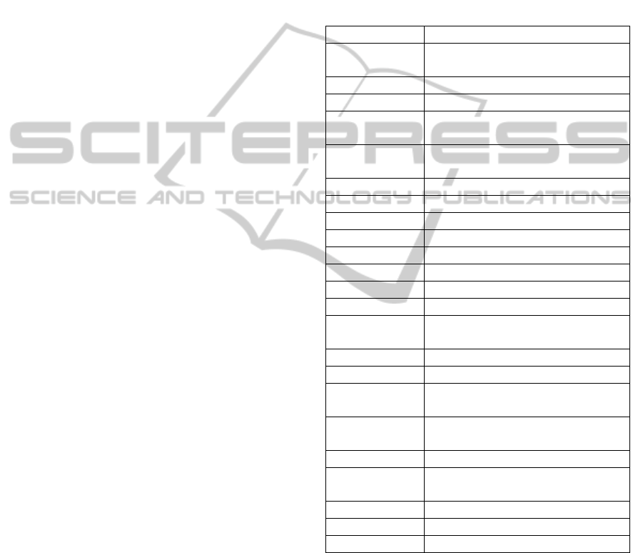
APPENDIX: ABBREVIATION

Abbreviation Full Name

CHCP

Centralized Heating and Cooling

Plant

Carbon Dioxide

CoGen Cogeneration

DGEI

Decision-Guided Energy

Investment

DVPC

Dominion Virginia Power

Company

EC EnergyConnect

ECU Energy Contractual Utility

EFD Energy Future Demand

EFE Energy Facility Expansion

EGP Energy Generation Process

EHD Energy Historical Demand

ES Electricity Supply

FCWA Fairfax County Water Authority

FMD

Facilities Management

Department

GHG Greenhouse Gas

GMU George Mason University

MILP

Mixed Integer Linear

Programming

MINLP

Mixed Integer Non-Linear

Programming

Mono-Nitrogen Oxide

OPL

Optimization Programming

Language

QoS Quality of Service

ROI Return On Investment

WGLC Washington Gas Light Company

ADecision-GuidedEnergyFrameworkforOptimalPower,Heating,andCoolingCapacityInvestment

369