
Adaptive Filtering for Stochastic Volatility by using Exact Sampling
ShinIchi Aihara
1
, Arunabha Bagchi
2
and Saikat Saha
3
1
Department of Mechanical Systems, Tokyo University of Science Suwa, 5000-1 Toyohira, Chino, Nagano, Japan
2
Department of Applied Mathematics, Twente University, P.O.Box 217,7500AE, Ensched, The Netherlands
3
Department of Electrical Engineering, Lik¨oping University, SE-58183 Lik¨oping Sweden
Keywords:
Particle Filter, Stochastic Volatility, Parameter Identification, Adaptive Filter.
Abstract:
We study the sequential identification problem for Bates stochastic volatility model, which is widely used as
the model of a stock in finance. By using the exact simulation method, a particle filter for estimating stochastic
volatility is constructed. The systems parameters are sequentially estimated with the aid of parallel filtering
algorithm. To improve the estimation performance for unknown parameters, the new resampling procedure is
proposed. Simulation studies for checking the feasibility of the developed scheme are demonstrated.
1 INTRODUCTION
In the early 1960s, the linear filtering theory is formu-
lated by Kalman and Bucy (Kalman and Bucy, 1961)
and nonlinear filtering has already been well devel-
oped by many researchers, see Bensoussan (Bensous-
san, 1992) and the bibliography therein. The realiza-
tion problem for the nonlinear filter is still not easy.
The recent development of particle filtering theory
(Doucet et al., 2000) enable us to realize the nonlin-
ear filtering in an easy way with the aid of the digital
computer.
In this paper we consider the Bates model which
is used in the fiance problem. In this model, we ob-
serve the tick value of stock price and need to esti-
mate the movement of the volatility process for trad-
ing the stock and/or options. It is not possible to apply
the nonlinear filtering theory to this volatility estima-
tion problem, because this is out of the usual filter-
ing problem in the continuous stochastic systems (Ai-
hara and Bagchi, 2006). To circumvent this difficulty,
the particle filter theory is usually applied in (Aihara
et al., 2008; Capp´e et al., 2005; Javaheri, 2005). The
Bates model is given by
dS
t
= µ
S
S
t
dt +
√
v
t
S
t
dB
t
+ S
t
dZ
J
t
−λm
J
S
t
dt, (1)
dv
t
= κ(θ−v
t
)dt + ξ
√
v
t
dZ
t
(2)
where B
t
and Z
t
are standard Brownian motion pro-
cesses with correlation ρ and Z
J
t
denotes the pure-
jump process. Noting that the process S
t
denotes
the stock value, the observation data y
t
= logS
t
/S
0
is given by
dy
t
= (µ
S
−λm
J
−
1
2
v
t
)dt +
√
v
t
dB
t
+ dq
J
t
, (3)
where q
J
t
is a compound Poisson process with in-
tensity λ and Gaussian distribution of jump size,i.e.,
N(µ
J
,σ
2
J
), and the mean relative jump size is given
by m
J
= E(exp(U
s
) −1) = exp(µ
J
+ σ
2
J
/2) −1 and
where the λm
J
S
t
term in (1) compensates for the in-
stantaneous change in expected stock introduced by
the pure-jump process Z
J
t
. The particular properties
of this model are
1. The observation mechanism (3) contains the sig-
nal dependent noise.
2. The observation noise has a correlation with the
systems noise.
From the first property, the estimation of stochastic
volatility becomes out of filtering problem. To cir-
cumvent this difficulty, all systems are discretized and
the particle filter is applied in (Aihara et al., 2008;
Johannes and Polson, 2006). However the usual dis-
cretization method transformed the original continu-
ous non-Gaussian system into the conditional Gaus-
sian. Recently, Brodie and Kaya (Broadie and Kaya,
2006; Smith, 2008; van Haastrecht and Pelsser, 2010)
proposed the exact simulation method from the fact
that the original system has a non-central chi-square
distribution and we use this technique to the particle
filtering (Aihara et al., 2012). Introducing the new
Brownian motion
˜
Z
t
=
1
p
1−ρ
2
(Z
t
−ρB
t
), (4)
326
Aihara S., Bagchi A. and Saha S..
Adaptive Filtering for Stochastic Volatility by using Exact Sampling.
DOI: 10.5220/0004454703260335
In Proceedings of the 10th International Conference on Informatics in Control, Automation and Robotics (ICINCO-2013), pages 326-335
ISBN: 978-989-8565-70-9
Copyright
c
2013 SCITEPRESS (Science and Technology Publications, Lda.)

from the second property, (2) becomes
dv
t
= κ(θ−v
t
)dt + ξ
√
v
t
q
1−ρ
2
d
˜
Z
t
+ξρ(dy
t
−(µ
S
−λm
J
−
1
2
v
t
)dt −dq
J
t
). (5)
Although in (Aihara et al., 2012) the exact particle fil-
tering procedure has been applied to the systems (5)
and (3), the priority property of the exact simulation
method can not be guaranteed and the final parameter
estimation results are not satisfactory. In this paper,
we introduce the rejection and acceptance method for
enjoying the exact simulation method and construct
the parallel filtering algorithm with an new resam-
pling procedure for parameter identification.
In Sec. 2, we review the exact particle filtering
with the new use of rejection and resampling proce-
dure. For the real application to the finance problem,
the market price of risk terms are included in the orig-
inal dynamics in Sec. 3. Simulation studies for fil-
tering and smoothing are presented in Sec. 5. The
new parallel filter algorithm is developed for estimat-
ing the systems unknown parameters sequentially in
Sec. 4. Finally some simulation studies for parameter
estimation are presented in Sec. 6.
2 EXACT PARTICLE FILTERING
2.1 Exact Sampling
In order to perform the particle filter, the original
system is usually approximated to the discrete-time
one by using the Euler method. This approximation
easily causes bias from the original continuous sys-
tem. For example, the discrete-time volatility pro-
cess v
k
often becomes negative value. To avoid this
bias, we propose the exact sampling method which is
developed by Broadie and Kaya (Broadie and Kaya,
2006),Smith (Smith, 2008) and (van Haastrecht and
Pelsser, 2010) for simulating the Heston process. In
this paper, from (5) we can obtain the optimal impor-
tance function p(v
t
2
|v
t
1
,y
t
2
,y
t
1
). Hence we generate
samples from this optimal importance function. Now
we shall present the exact sampling procedure. For
simplicity we consider the time intervalt
1
< t
2
and set
the following assumption: At most one jump occurs
in this time interval and we observe y
t
2
and y
t
1
.
2.1.1 Exact Sampling from p(v
t
2
|v
t
1
,y
t
2
,y
t
1
)
From (1), the volatility process v
t
2
is represented by
v
t
2
= ˜v
t
1
+
Z
t
2
t
1
˜
κ(
˜
θ−v
s
)ds
+
Z
t
2
t
1
ξ
√
v
s
q
1−ρ
2
d
˜
Z
s
, (6)
where
˜v
t
1
= v
t
1
+ ρξ{y
t
2
−y
t
1
−(µ
S
−λm
J
)(t
2
−t
1
) −∆q
i
t
1
}
˜
κ = κ−
ρξ
2
˜
θ =
κθ
˜
κ
∆q
i
t
1
= jump sample from q
J
t
for t
1
< t < t
2
.
Now assuming that ˜v
t
1
≥0, we find that the transition
law of v
t
2
given by v
t
1
,y
t
1
and y
t
2
is expressed as the
non-central chi-square random variable χ
2
d
(λ
χ
) with d
degrees of freedom and non-centrality parameter λ
χ
,
ξ
2
(1−ρ
2
)(1−e
−
˜
κ(t
2
−t
1
)
)
4
˜
κ
χ
2
d
(λ
χ
), (7)
where
d =
4
˜
θ
˜
κ
ξ
2
(1−ρ
2
)
and
λ
χ
=
4
˜
κe
−
˜
κ(t
2
−t
1
)
ξ
2
(1−ρ
2
)(1−e
−
˜
κ(t
2
−t
1
)
)
˜v
t
1
.
Hence by using MATLAB code ”ncx2rnd.m”, we can
get a sample v
t
2
.
For the case that ˜v
t
1
< 0, this event may occur
when v
t
1
is very small in generating particles by using
the data y
t
2
−y
t
1
. In the real world, we have already
get the value y
t
2
−y
t
1
. Hence v
t
1
should satisfy
v
t
1
+ ρξ{y
t
2
−y
t
1
−(µ
S
−λm
J
)(t
2
−t
1
) −∆q
i
t
1
}
+
˜
κ
˜
θ(t
2
−t
1
) ≥ 0. (8)
2.1.2 ˜v
t
1
< 0 Case
We use the rejection and resampling procedure. At the
time t
1
, we already get many particles say v
(i)
t
1
. Hence
we check the above inequality (8) for each v
(i)
t
1
. If the
particles which do not satisfy (8) are found, we ignore
these and perform a resampling procedure.
2.2 Construction of Probability Density
Function
If we use the Euler scheme for discretization, the
generated sample becomes the conditionally Gaus-
sian. However for the exact sampling scheme , the
AdaptiveFilteringforStochasticVolatilitybyusingExactSampling
327

processes generated are governed by the non-central
chi-square distribution. Although the explicit func-
tion form of this distribution is not possible, we can
numerically evaluate the pdf by using the MATLAB
code, ”ncx2pdf.m”.
• p(v
t
2
|v
t
1
,y
t
2
,y
t
1
) form
Noting that the jump occurs at most one time dur-
ing the time interval [t
2
,t
1
], i.e, the probability
that the jump occurs is λe
−λ(t
2
−t
1
)
and no jump
becomes 1 −λe
−λ(t
2
−t
1
)
, and the jump size U
s
·
is
Gaussian with mean µ
J
and variance σ
2
J
, we have
p(v
t
2
|v
t
1
,y
t
2
,y
t
1
)
= (1−e
−λ(t
2
−t
1
)
λ(t
2
−t
1
))
× p(v
t
2
|v
t
1
,y
t
2
,y
t
1
,∆q
j
t
1
= 0)
+ e
−λ(t
2
−t
1
)
λ(t
2
−t
1
)
Z
∞
−∞
p(v
t
2
|v
t
1
,y
t
2
,y
t
1
,U
s
)
1
q
2πσ
2
J
exp(−
(U
s
−µ
J
)
2
2σ
2
J
)dU
s
= (1−e
−λ(t
2
−t
1
)
λ(t
2
−t
1
))
×pdf of
(
ξ
2
(1−ρ
2
)(1−e
−
˜
κ(t
2
−t
1
)
)
4
˜
κ
χ
2
d
(
˜
λ
χ
)
)
+ e
−λ(t
2
−t
1
)
λ(t
2
−t
1
)
×
Z
∞
−∞
pdf of
(
ξ
2
(1−ρ
2
)(1−e
−
˜
κ(t
2
−t
1
)
)
4
˜
κ
×χ
2
d
(
˜
λ
χ
−
4
˜
κe
−
˜
κ(t
2
−t
1
)
ρ
ξ(1−ρ
2
)(1−e
−
˜
κ(t
2
−t
1
)
)
U
s
)
)
×
1
q
2πσ
2
J
exp(−
(U
s
−µ
J
)
2
2σ
2
J
)dU
s
(9)
where
˜
λ
χ
=
4
˜
κe
−
˜
κ(t
2
−t
1
)
ξ
2
(1−ρ
2
)(1−e
−
˜
κ(t
2
−t
1
)
)
×{v
t
1
+ ρξ{y
t
2
−y
t
1
−(µ
S
−λm
J
)(t
2
−t
1
)}}
In (9), the first term implies that we have no jump
and the second term is caused from the jump size
U
s
∈N(µ
J
,σ
2
J
).
• p(v
t
2
|v
t
1
,y
t
1
) form
It follows from (2) that
p(v
t
2
|v
t
1
,y
t
1
) = pdf of
ξ
2
(1−e
−κ(t
2
−t
1
)
)
4κ
χ
2
˜
d
(λ
v
χ
),
where
˜
d =
4θκ
ξ
2
,
and
λ
v
χ
=
4κe
−κ(t
2
−t
1
)
ξ
2
(1−e
−κ(t
2
−t
1
)
)
v
t
1
.
• p(y
t
2
|y
t
1
,
R
t
2
t
1
v
s
ds) form
In this case, from
dy
t
= (µ
S
−λm
J
−
1
2
v
t
)dt +
ρ
ξ
(dv
t
−κ(θ−v
t
)dt)
+
q
1−ρ
2
√
v
t
d
˜
Z
t
+ dq
J
t
we easily get
p(y
t
2
|y
t
1
,
Z
t
2
t
1
v
s
ds) =
1−e
−λ(t
2
−t
1
)
λ(t
2
−t
1
)
q
2π(1−ρ
2
)
R
t
2
t
1
v
s
ds
×exp[−
1
2(1−ρ
2
)
R
t
2
t
1
v
s
ds
{y
t
2
−[y
t
1
+ (µ
S
−λm
J
−
κρθ
ξ
)(t
2
−t
1
)
−(
1
2
−
κρ
ξ
)
Z
t
2
t
1
v
s
ds+
ρ
ξ
(v
t
2
−v
t
1
)]}
2
]
+
e
−λ(t
2
−t
1
)
λ(t
2
−t
1
)
q
2π((1−ρ
2
)
R
t
2
t
1
v
s
ds+ σ
2
J
)
×exp[−
1
2((1−ρ
2
)
R
t
2
t
1
v
s
ds+ σ
2
J
)
{y
t
2
−[y
t
1
+ (µ
S
−λm
J
−
κρθ
ξ
)(t
2
−t
1
)
−(
1
2
−
κρ
ξ
)
Z
t
2
t
1
v
s
ds+ µ
J
+
ρ
ξ
(v
t
2
−v
t
1
)]}
2
]
(10)
2.3 Exact Particle Filter Algorithm
Now we can perform the exact particle filter. The
weight w
(i)
·
is given by the following recursive form:
for i = 1,··· , N and k = 1,··· ,m
w
(i)
t
k
= w
(i)
t
k−1
p(y
t
k
|y
t
k−1
,
R
t
k
t
k−1
v
(i)
s
ds)p(v
(i)
t
k
|v
(i)
t
k−1
)
p(v
(i)
t
k
|v
(i)
t
k−1
,y
t
k
,y
t
k−1
)
. (11)
Of course we need to perform the resampling
scheme in the above filtering algorithm.
It is also possible to construct the smoothing algo-
rithm by using forward filtering-backward sampling
scheme by Doucet et. al. (Doucet et al., 2000)
Algorithm(Sample realization).
• Run the particle filter to obtain
(v
(i)
t
k
,ω
(i)
t
k
)
1≤k≤m,1≤i≤N
.
• By using the systematic resampling method, we
generate new index J
m
from {ω
(i)
t
m
}
1≤i≤N
.
ICINCO2013-10thInternationalConferenceonInformaticsinControl,AutomationandRobotics
328

• Set ˜v
(i)
t
m
as v
J
m
t
m
.
• For k = m−1 to 1;
Resample to get J
k
from
{ω
(i)
t
k
p( ˜v
(i)
t
k
+1
|v
(i)
t
k
)}
1≤i≤N
.
Set ˜v
(i)
t
k
as v
J
k
k
.
• ˜v
(i)
= [ ˜v
(i)
t
1
, ˜v
(i)
t
2
,··· , ˜v
(i)
t
m
] is the realized particles for
smoothing with 1/N probability.
3 MARKET PRICE OF RISK
For estimation we also need the dynamics of the state
S
t
and v
t
under the actual probability measure P . We
specify the market price of risk for B
t
and Z
t
as
d
B
P
t
Z
P
t
= d
B
t
Z
t
−
λ
S
√
v
t
0
0 λ
v
√
v
t
dt.
We ignore the jump-timing risk premium and the
jump-size risk is assumed to be included in µ
J
. Now
the dynamics of y
t
and v
t
under P is given by
dy
t
= (µ
S
−λm
J
+ (λ
S
−
1
2
)v
t
)dt +
√
v
t
dB
P
t
+ dq
J
t
dv
t
= (κθ−(κ−λ
v
ξ)v
t
)dt + ξ
√
v
t
q
1−ρ
2
d
˜
Z
P
t
+ ξρ(dy
t
−(µ
S
−λm
J
−(
1
2
−λ
S
)v
t
)dt −dq
J
t
).
Hence it is possible to apply our particle filer algo-
rithm to this world measure dynamics. The corre-
sponding dynamics is transformed to
v
t
2
= ˜v
t
1
+
Z
t
2
t
1
˜
κ(
˜
θ−v
s
)ds+
Z
t
2
t
1
ξ
√
v
s
q
1−ρ
2
d
˜
Z
s
,
where
˜v
t
1
= v
t
1
+ ρξ{y
t
2
−y
t
1
−(µ
S
−λm
J
)(t
2
−t
1
) −∆q
i
t
1
}
˜
κ = κ−
ρξ
2
+ ξ(ρλ
S
−λ
v
)
˜
θ =
κθ
˜
κ
.
p(v
t
2
|v
t
1
) becomes
p(v
t
2
|v
t
1
) = pdf of
ξ
2
(1−e
−(κ−ξλ
v
)(t
2
−t
1
)
)
4(κ−ξλ
v
)
χ
2
d
(λ
v
χ
),
where
d =
4θκ
ξ
2
,
and
λ
v
χ
=
4(κ−ξλ
v
)e
−(κ−ξλ
v
)(t
2
−t
1
)
ξ
2
(1−e
−(κ−ξλ
v
)(t
2
−t
1
)
)
v
t
1
.
Noting that
dy
t
= (µ
S
−λm
J
+ (λ
S
−
1
2
)v
t
)dt
+
ρ
ξ
(dv
t
−κθdt + (κ −λ
v
ξ)v
t
)dt)
+
q
1−ρ
2
√
v
t
d
˜
Z
t
+ dq
J
t
,
we also have
p(y
t
2
|y
t
1
,
Z
t
2
t
1
v
s
ds) =
1−e
−λ(t
2
−t
1
)
λ(t
2
−t
1
)
q
2π(1−ρ
2
)
R
t
2
t
1
v
s
ds
×exp[−
1
2(1−ρ
2
)
R
t
2
t
1
v
s
ds
{y
t
2
−[y
t
1
+ (µ
S
−λm
J
−
κρθ
ξ
)(t
2
−t
1
)
−(
1
2
−
κρ
ξ
+ ρλ
v
−λ
S
)
Z
t
2
t
1
v
s
ds+
ρ
ξ
(v
t
2
−v
t
1
)]}
2
]
+
e
−λ(t
2
−t
1
)
λ(t
2
−t
1
)
q
2π((1−ρ
2
)
R
t
2
t
1
v
s
ds+ σ
2
J
)
×exp[−
1
2((1−ρ
2
)
R
t
2
t
1
v
s
ds+ σ
2
J
)
{y
t
2
−[y
t
1
+ (µ
S
−λm
J
−
κρθ
ξ
)(t
2
−t
1
)
−(
1
2
−
κρ
ξ
+ ρλ
v
−λ
S
)
Z
t
2
t
1
v
s
ds+ µ
J
+
ρ
ξ
(v
t
2
−v
t
1
)]}
2
]
4 SIMULATION STUDIES FOR
FILTERING AND SMOOTHING
In this section, we simulate the proposed filtering and
smoothing equations with known systems parameters
for Heston model without any market price of risk
terms for simplicity.
The systems parameters are listed in Table-1 and
in this case the point ”zero” is acceptable.
Table 1: Model parameters.
κ θ µ
S
ρ ξ
True 0.8638 1.0000 0.0100 -0.1050 2.5017
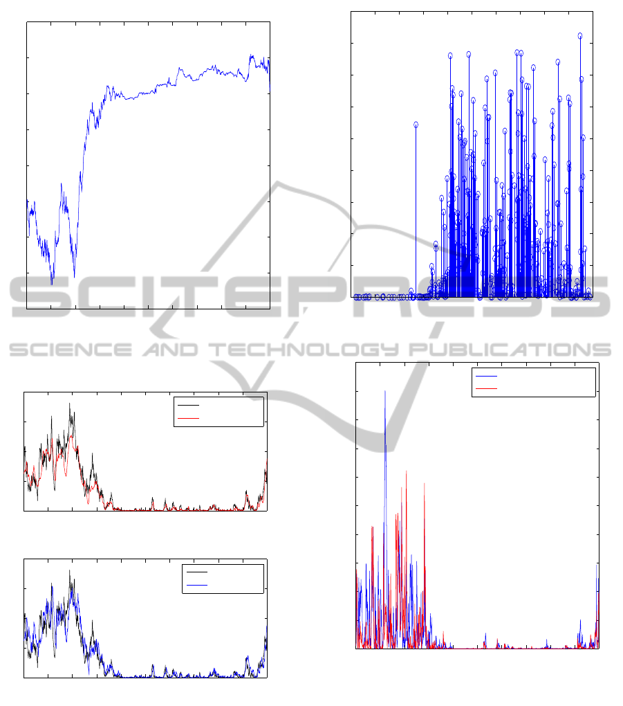
We present the log price in Fig.1. As shown in
Fig.2, the volatility process hits ”zero” at many times
because the degree of freedoms is less than 2. The
rejection and resampling rate is shown in Fig.3.
AdaptiveFilteringforStochasticVolatilitybyusingExactSampling
329
0 0.1 0.2 0.3 0.4 0.5 0.6 0.7 0.8 0.9 1
−0.3
−0.2
−0.1
0
0.1
0.2
0.3
0.4
0.5
Log price
Time (year)
Log Price
Figure 1: Observation data y
t
.
0 0.1 0.2 0.3 0.4 0.5 0.6 0.7 0.8 0.9 1
0
0.2
0.4
0.6
0.8
True value and estimated value of volatility
Time (year)
Volatility
True value
Smoothed estimate
0 0.1 0.2 0.3 0.4 0.5 0.6 0.7 0.8 0.9 1
0
0.2
0.4
0.6
0.8
True value and estimated value of volatility
Time (year)
Volatility
True value
Filtered estimate
Figure 2: True and estimated v
t
.
5 PARALLEL FILTERING
ALGORITHM
In a market, traders buy or sell stocks from their feel-
ing of the volatility movement of the traded stock.
Form this fact, we need to estimate the volatility itself
0 0.1 0.2 0.3 0.4 0.5 0.6 0.7 0.8 0.9 1
0
0.1
0.2
0.3
0.4
0.5
0.6
0.7
0.8
0.9
Time (year)
Rejection and resampling rate
Figure 3: Rejection and resampling rate.
0 0.1 0.2 0.3 0.4 0.5 0.6 0.7 0.8 0.9 1
0
0.01
0.02
0.03
0.04
0.05
0.06
0.07
0.08
0.09
0.1
Time (year)
Exact square error
Filter case:sum =4.0674
Smoothing case : sum=3.0109
Figure 4: Mean square errors.
rather than the parameters in the model. The estimate
of the volatility should be online. Hence, in this sec-
tion, we construct the recursiveonline estimate for the
volatility. Of course to obtain the estimate of volatil-
ity, we also get the estimate of systems parameters at
the same time. Here the unknown parameters are de-
noted by
α = [κ,θ,ν
S
,ρ,ξ,λ,ν
J
,σ
J
,λ
v
,λ
S
].
Now we set candidates of unknown parameter α such
ICINCO2013-10thInternationalConferenceonInformaticsinControl,AutomationandRobotics
330

that
α
( j)
∈ uniformly random vectors in Θ, j = 1,··· ,M
p
If we know an a-priori information for Θ, we may
set the pdf p
o
(α). For each α
( j)
, we solve the par-
ticle filter ˆv
t
k
(α
( j)
) from Section 2.3. Hence from
(B.D.O.Anderson and J.B.Moore, 1979), we get the
posteriori density given by
p(α
( j)
|y
t
0
:t
k
)
=
{Σ
N
i=1
w
(i)
t
k−1
(α
( j)
)LF
k,i
}p(α
( j)
|y
t
0
:t
k−1
)
Σ
M
p
j=1
n
{Σ
N
i=1
w
(i)
t
k−1
(α
( j)
)LF
k,i
}p(α
( j)
|y
t
0
:t
k−1
)
o
where
LF
k,i
= p(y
k
|y
k−1
,
Z
t
k
t
k−1
v
(i)
s
(α
( j)
)ds).
The estimates of volatility and parameters are given
by
ˆv
k
= Σ
M
p
j=1
ˆv
t
k
(α
( j)
)p(α
( j)
|y
t
0
:t
k
) (12)
ˆ
α
k
= Σ
M
p
j=1
α
( j)
p(α
( j)
|y
t
0
:t
k
). (13)
5.1 New Resampling Procedure
The sample of parameter {α
( j)
}
M
P
j=1
is drawn only
from the initial information (in this paper we set the
uniform distribution). Hence for a long time period
the estimates of parameters are sometimes stacked
with some biases. This may cause from the fact that
there are so many unknown parameters while we get
a scaler observation data. In order to improve this
property, a resampling for the candidates for param-
eters α
( j)
is usually performed in MCMC algorithm
in (Johannes and Polson, 2006). In the parallel filter-
ing algorithm, we already get the posterior probability
p(α
( j)
|y
t
0
:t
k
) and from this distribution, we propose to
get new samples for α
( j)
by using the following pro-
cedure:
1. We set the resampling time t
r
p
if
(
M
P
∑
j=1
p
2
(α
( j)
|y
t
0
:t
r
p
))
−1
≤
2M
P
3
,
we generate new sample α
( j)
from the step 2) to
6).
2. Calclulate
ˆ
α
t
r
p
= Σ
M
p
j=1
α
( j)
p(α
( j)
|y
t
0
:t
r
p
)
ˆ
σ
α(i)
= Σ
M
p
j=1
(α
( j)
(i))
2
p(α
( j)
(i)|y
t
0
:t
r
k
) −(
ˆ
α
( j)
t
r
p
(i))
2
for i = 1,2,··· ,10.
3. We denote the parameter range at the resampling
time point t = t
r
p
as
lb(i,t
r
p
) ≤ α(i) ≤ ub(i,t
r
p
) for i = 1,2,··· ,10,
where lb(i,t) = lb(i) and ub(i,t) = ub(i) for t <
the first resampling time.
4. From the calculated
ˆ
α
t
r
p
and
ˆ
σ
α
, we reset the pa-
rameter range from t
r
p−1
as
lb(i,t
r
p
) = max(lb(i,t
r
p−1
),
ˆ
α
t
r
k
(i) −3
ˆ
σ
α(i)
)
and
ub(i,t
r
p
) = min(ub(i,t
r
p−1
),
ˆ
α
t
k
p
+ 3
ˆ
σ
α(i)
).
5. Construct the candidates of parameter k;
α
k
(i) = lb(i,t
r
p
) +
ub(t
r
p
) −ub(t
r
p
)
M
p
−1
(i−1).
for k = 1,2,··· ,M
p
.
6. Construct the posterior distribution for each pa-
rameter α(i) by using the Gaussian approxima-
tion:
P(α(i)|y
t
0
:t
r
p
) ∼ N (α(i);
ˆ
α
t
r
p
,ε
i
ˆ
σ
1/2
α(i)
),
where ε
i
is a user defined parameter to increase
diversity.
7. Allocate n
k
copies of the particle α
k
(i) from
n
i
= the number of
(k−1) + ˜u
M
p
∈ (F
G
(α
k−1
(i)),F
G
(α
k
(i))]
for ˜u= uniform random number, where F
G
is an
approximated Gaussian distribution (step 6)):
F
G
(α
k
(i))
=
R
α
k
(i)
−∞
1
√
2πε
i
ˆ
σ
α(i)
exp[−
1
2(ε
i
ˆ
σ
α
(i))
2
(α(i) −
ˆ
α
t
r
p
)
2
]dα(i)
F
G
(lb(i,t
r
p
))
.
8. Construct new candidate; for j = 1,2, ··· , M
P
α
( j)
= [α
j
(1),α
j
(2),··· ,α
j
(10)].
9. Reset p(α
( j)
|y
y
0
:t
r
p
) = 1/M
P
.
6 SIMULATION STUDIES
We set the following parameters in Table 2.
The lower and upper bounds for parameters are set as
Here we set dt = 0.001, T = 1,M = 100,M
P
= 60 and
t
r
= 20dt,ε
1
= 1.1, ε
2
= 1.1,ε
3
= 1.15,ε
4
= 1.01,ε
5
=
1.01, ε
6
= 1.15,ε
7
= 1.15,ε
8
= 1.15,ε
9
= 1.15, and
ε
10
= 1.15. In Fig.5, we show the true volatility state
AdaptiveFilteringforStochasticVolatilitybyusingExactSampling
331
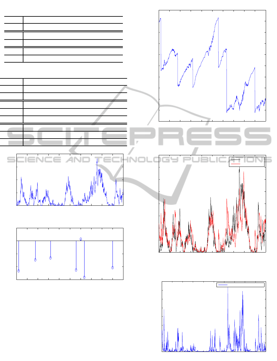
Table 2: Model parameters.
κ θ µ
S
ρ
True 0.8638 1.1000 0.6000 -0.1500
ξ λ µ
J
σ
J
True 2.1017 5.4000 -0.3000 0.2500
λ
v
λ
S
True 0.1882 0.1723
Table 3: Lower and upper bounds of model parameters.
κ θ µ
S
ρ
Upper 1.6412 2.0900 1.140 -0.001
Lower 0.0086 0.0011 0.006 -0.300
ξ λ µ
J
σ
J
Upper 3.9932 10.260 -0.0030 0.4570
Lower 0.0210 0.0540 -0.5700 0.0025
λ
v
λ
S
Upper 0.35758 0.62174
Lower 0.0018 0.0032
0 0.1 0.2 0.3 0.4 0.5 0.6 0.7 0.8 0.9 1
0
0.1
0.2
0.3
0.4
Time (year)
Volatility v
0 0.1 0.2 0.3 0.4 0.5 0.6 0.7 0.8 0.9 1
−0.6
−0.4
−0.2
0
0.2
Time (year)
Compoud Poisson process
Figure 5: The true volatility state and compound Poisson
process.
and compound Poisson process. The observed log
price is also shown in Fig.6. The estimated volatil-
ity is shown in Fig.7 with the square error in Fig.8.
We also present the resampling rates of the parti-
cle filter of this algorithm in Fig. 9.
The estimates of unknown parameters are demon-
strated from Figs 10 to 19 with the corresponding his-
togram for 0 ≤t ≤ 1.
The true and estimated parameters at t = 1 are
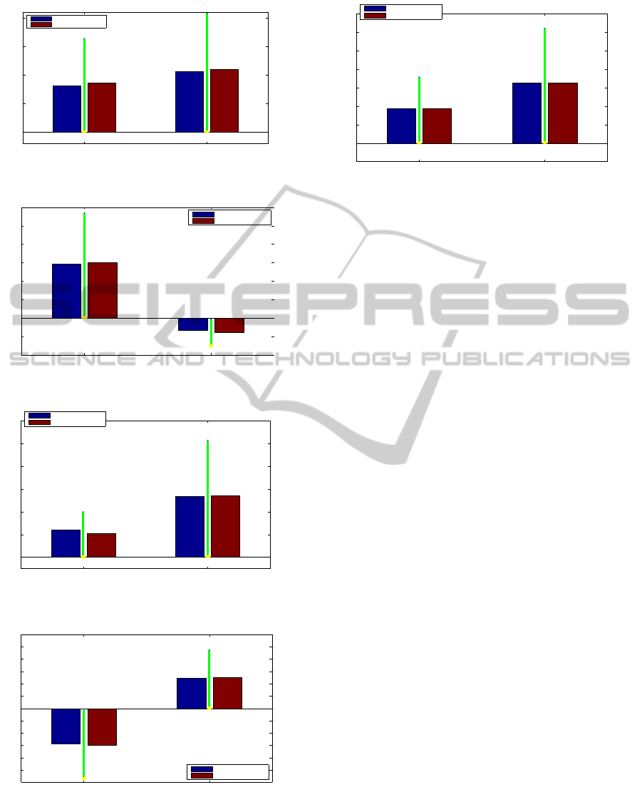
shown in Figs. 20-24 where the green line indicated
0 0.1 0.2 0.3 0.4 0.5 0.6 0.7 0.8 0.9 1
−0.9
−0.8
−0.7
−0.6
−0.5
−0.4
−0.3
−0.2
−0.1
0
0.1
Time (year)
Log price
Figure 6: Observed log price.
0 0.1 0.2 0.3 0.4 0.5 0.6 0.7 0.8 0.9 1
0
0.05
0.1
0.15
0.2
0.25
0.3
0.35
0.4
True value and estimated value of volatility
Time (year)
Volatility
True value
Filtered state1.1
Figure 7: True and estimated volatility.
0 0.1 0.2 0.3 0.4 0.5 0.6 0.7 0.8 0.9 1
0
0.005
0.01
0.015
0.02
0.025
0.03
0.035
0.04
Time (year)
Exact square error
Square error:sum =2.3106
Figure 8: Square error of estimated volatility.
the upper and lower bounds for each parameters at
t = 0.
ICINCO2013-10thInternationalConferenceonInformaticsinControl,AutomationandRobotics
332
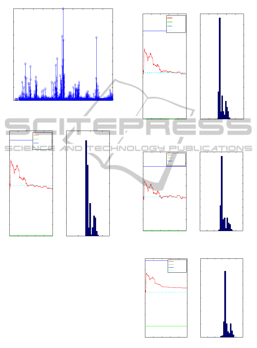
0 0.1 0.2 0.3 0.4 0.5 0.6 0.7 0.8 0.9 1
0
0.1
0.2
0.3
0.4
0.5
0.6
0.7
Time (year)
Rejection and resampling rate
Figure 9: Square error of estimated volatility
0 0.2 0.4 0.6 0.8 1
0
0.2
0.4
0.6
0.8
1
1.2
1.4
1.6
1.8
Time (year)
True and estimated parameters
κ
Estimated value
Lower bound
Upper bound
True value
0 0.5 1 1.5
0
50
100
150
200
250
300
350
400
Parameter
Mean =0.935
Cov. =1.8e−02
Figure 10: Estimated κ and histogram for 0 ≤t ≤ 1
7 CONCLUSIONS
By using the non-central chi-square random genera-
tion method, we developed the particle filter for esti-
mating the stochastic volatility process. The sequen-
tial estimation for the systems unknown parameters
are performed with the aid of the new resampling pro-
cedure. In this procedure, we need to choose the re-
sampling time t
r
and the user defined parameter ε
i
to
obtain the good numerical results. This turning prob-
lem is still an open problem.
0 0.2 0.4 0.6 0.8 1
0
0.5
1
1.5
2
2.5
Time (year)
True and estimated parameters
θ
Estimated value
Lower bound
Upper bound
True value
0 0.5 1 1.5 2 2.5
0
50
100
150
200
250
300
350
400
450
500
Parameter
Mean =1.22
Cov. =2.7e−02
Figure 11: Estimated θ and histogram for 0 ≤ t ≤ 1
0 0.2 0.4 0.6 0.8 1
0
0.2
0.4
0.6
0.8
1
1.2
1.4
Time (year)
True and estimated parameters
µ
S
Estimated value
Lower bound
Upper bound
True value
0 0.2 0.4 0.6 0.8 1 1.2
0
50
100
150
200
250
300
350
400
450
500
Parameter
Mean =0.651
Cov. =6.1e−03
Figure 12: Estimated µ and histogram for 0 ≤ t ≤ 1.
0 0.2 0.4 0.6 0.8 1
−0.35
−0.3
−0.25
−0.2
−0.15
−0.1
−0.05
0
Time (year)
True and estimated parameters
ρ
Estimated value
Lower bound
Upper bound
True value
−0.25 −0.2 −0.15 −0.1 −0.05 0
0
100
200
300
400
500
600
Parameter
Mean =−0.118
Cov. =3.5e−04
Figure 13: Estimated ρ and histogram for 0 ≤t ≤ 1.
AdaptiveFilteringforStochasticVolatilitybyusingExactSampling
333
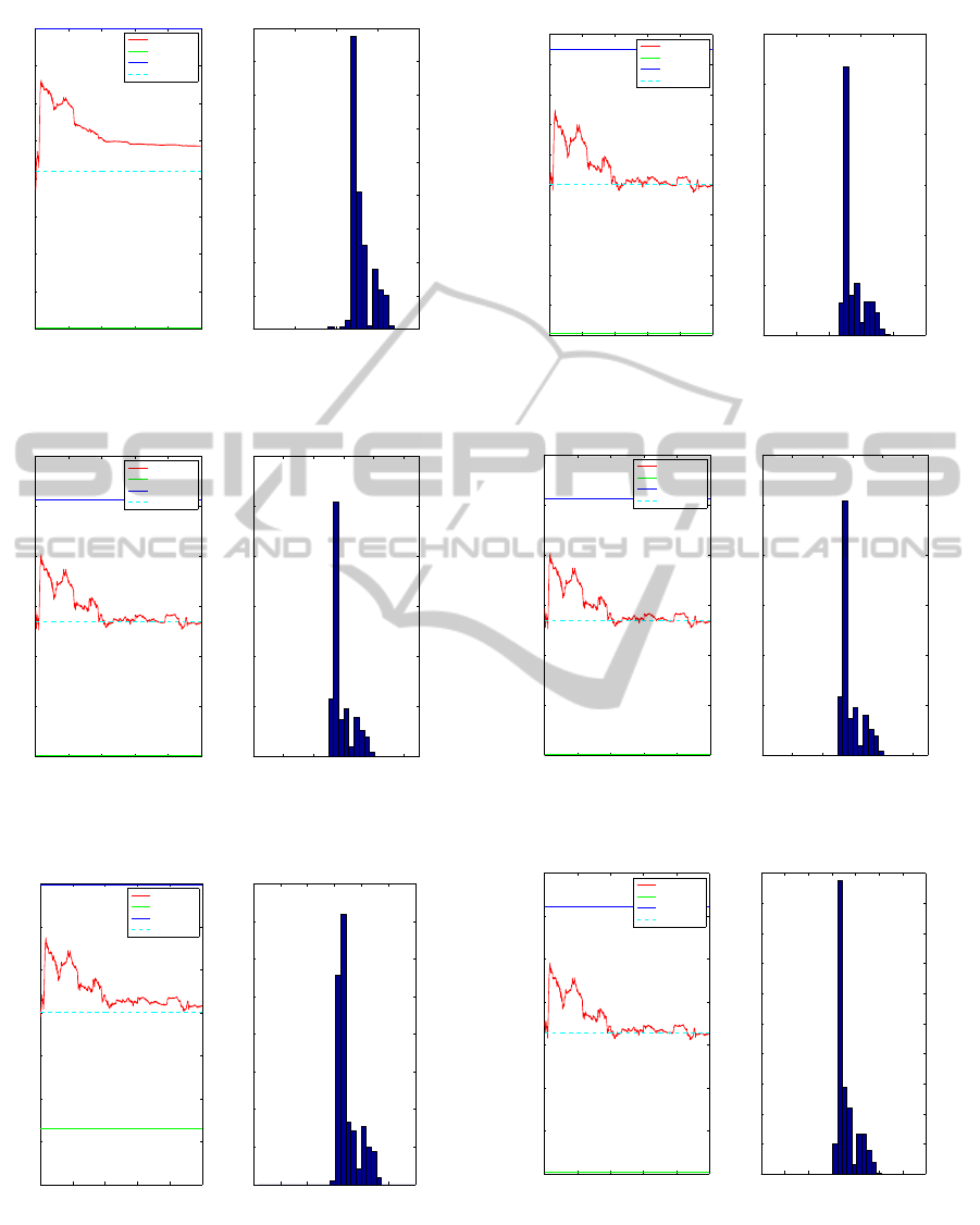
0 0.2 0.4 0.6 0.8 1
0
0.5
1
1.5
2
2.5
3
3.5
4
Time (year)
True and estimated parameters
ξ
Estimated value
Lower bound
Upper bound
True value
0 1 2 3 4
0
50
100
150
200
250
300
350
400
450
Parameter
Mean =2.61
Cov. =6.2e−02
Figure 14: Estimated ξ and histogram for 0 ≤t ≤ 1.
0 0.2 0.4 0.6 0.8 1
0
2
4
6
8
10
12
Time (year)
True and estimated parameters
λ
Estimated value
Lower bound
Upper bound
True value
0 2 4 6 8 10
0
100
200
300
400
500
600
Parameter
Mean =5.88
Cov. =4.7e−01
Figure 15: Estimated λ and histogram for 0 ≤t ≤ 1
0 0.2 0.4 0.6 0.8 1
−0.7
−0.6
−0.5
−0.4
−0.3
−0.2
−0.1
0
Time (year)
True and estimated parameters
µ
J
Estimated value
Lower bound
Upper bound
True value
−0.5 −0.4 −0.3 −0.2 −0.1 0
0
50
100
150
200
250
300
350
400
Parameter
Mean =−0.251
Cov. =1.6e−03
Figure 16: Estimated µ
J
and histogram for 0 ≤t ≤ 1
0 0.2 0.4 0.6 0.8 1
0
0.05
0.1
0.15
0.2
0.25
0.3
0.35
0.4
0.45
0.5
Time (year)
True and estimated parameters
σ
J
Estimated value
Lower bound
Upper bound
True value
0 0.1 0.2 0.3 0.4 0.5
0
100
200
300
400
500
600
Parameter
Mean =0.274
Cov. =1.0e−03
Figure 17: Estimated σ
J
and histogram for 0 ≤t ≤ 1
0 0.2 0.4 0.6 0.8 1
0
2
4
6
8
10
12
Time (year)
True and estimated parameters
λ
Estimated value
Lower bound
Upper bound
True value
0 2 4 6 8 10
0
100
200
300
400
500
600
Parameter
Mean =5.88
Cov. =4.7e−01
Figure 18: Estimated λ
v
and histogram for 0 ≤t ≤ 1
0 0.2 0.4 0.6 0.8 1
0
0.1
0.2
0.3
0.4
0.5
0.6
0.7
Time (year)
True and estimated parameters
λ
S
Estimated value
Lower bound
Upper bound
True value
0 0.1 0.2 0.3 0.4 0.5 0.6 0.7
0
50
100
150
200
250
300
350
400
450
500
Parameter
Mean =0.359
Cov. =1.7e−03
Figure 19: Estimated λ
S
and histogram for 0 ≤t ≤ 1
ICINCO2013-10thInternationalConferenceonInformaticsinControl,AutomationandRobotics
334
1 2
0
0.5
1
1.5
2
at T=1
κ θ
Estimated value
True value
Figure 20: Estimated κ and θ at t = 1.
1 2
−0.4
−0.2
0
0.2
0.4
0.6
0.8
1
1.2
at T=1
µ
S
ρ
Estimated value
True value
Figure 21: Estimated µ
S
and ρ at t = 1.
1 2
0
2
4
6
8
10
12
at T=1
ξ λ
Estimated value
True value
Figure 22: Estimated ξ and λ at t = 1.
1 2
−0.5
−0.4
−0.3
−0.2
−0.1
0
0.1
0.2
0.3
0.4
0.5
at T=1
µ
J
σ
J
Estimated value
True value
Figure 23: Estimated ξ and λ at t = 1.
1 2
−0.1
0
0.1
0.2
0.3
0.4
0.5
0.6
at T=1
λ
v
λ
S
Estimated value
True value
Figure 24: Estimated λ
V
and λ
S
at t = 1.
REFERENCES
Aihara, S. and Bagchi, A. (2006). Filtering and identifi-
cation of heston’s stochastic volatility and its market
risk. J. Economical Dynamics and Control, 30:2363–
2388.
Aihara, S., Bagchi, A., and S.Saha (2008). Estimating
volatility and model parameters of stochastic volatil-
ity models with jumps using particle filter. Proc. of
17th IFAC World Congress.
Aihara, S., Bagchi, A., and S.Saha (2012). Identification of
bates stochastic volatility model by using non-central
chi-square random generation method. Proc. of IEEE
ICASSP 2012.
B.D.O.Anderson and J.B.Moore (1979). Optimal Filtering.
Prentice-Hall, Inc., Englewood Cliffs, New Jersey.
Bensoussan, A. (1992). Stochastic Control of Partially Ob-
servable Systems. Cambridge University Press, Cam-
bridge.
Broadie, M. and Kaya, O. (2006). Exact simulation of
stochastic volatility and other affine jump diffusion
processes. Operations Research, 54(2):217–231.
Capp´e, O., E.Moulines, and Ryd´en, T. (2005). Inference in
Hidden Markov Models. Springer Science+Business
Media, Inc., New York.
Doucet, A., Godsil, S., and Andrieu, C. (2000). On se-
quential monte carlo sampling methods for bayesian
filtering. Statistics and Computing, 10:197–208.
Javaheri, A. (2005). Inside Volatility Arbitrage. John Wiley
& Sons, Inc, Hoboken.
Johannes, M. and Polson, N. (2006). MCMC method for
financial econometrics. In Y.Ait-Sahalia and Hansen,
L., editors, Handbook of Financial Econometrics. El-
sevier.
Kalman, R. and Bucy, R. (1961). New results in linear fil-
tering and prediction theory. Trans. ASME - Journ.
Basic Engineering, 83 (Series D):95–108.
Smith, R. (2008). An almost exact simulation method for
the heston model. Journal of Computational Finance,
11(1):115–125.
van Haastrecht, A. and Pelsser, A. (2010). Efficient, al-
most exact simulation of the heston stochastic volatil-
ity model. IJTAF, 13:1–43.
AdaptiveFilteringforStochasticVolatilitybyusingExactSampling
335
