
A Kalman Filter for Odometry using a Wheel Mounted Inertial Sensor
Bernd Gersdorf and Udo Frese
Cyber-Physical Systems, German Research Center for Artificial Intelligence, Bremen, Germany
Keywords:
Extended Kalman Filter (EKF), Odometry, Wheel, Sensor, Inertial Measurement Unit (IMU), MEMS,
Gyroscope, Accelerometer, Walker, Wheelchair, Tricycle, Navigation, ASSAM.
Abstract:
This paper describes an Extended Kalman Filter for a wheel mounted inertial measurement unit using two
accelerometers and a single gyroscope as a substitute for classical odometry sensing. The sensor can be
mounted with minimal effort on existing wheeled vehicles. It is highly robust against vibration while rolling
on uneven terrain and can cope with higher speeds even when the measurement range is partially exceeded.
It has been developed as a component of a GPS based urban navigation assistant for elderly people using
walkers, wheelchairs, or tricycles as an add-on device.
1 INTRODUCTION
Odometry is frequently used on wheeled robots as a
measurement of travelled distance. Incremental en-
coders are attached near the wheel or in the motor to
measure discrete angle steps interpreted as travelled
distance. Integrating such a sensor is easy when con-
sidered in the mechanical design from the beginning,
but adding an odometry sensor later on is often diffi-
cult. This is particular true for the application that mo-
tivates our research, where COTS (Commercial Off-
The-Shelf) wheelchairs or walkers shall be equipped
with odometry to give navigation support for elderly
people. An alternative is a sensor attached at an ar-
bitrary position on the wheel, that measures gravity
to derive a wheel angle. Accelerometer based sen-
sors are described by (Sonenblum, 2010) and (Huang
and Wang, 2011), both using cheap MEMS sensors on
tiny battery powered microcontroller boards for log-
ging or wireless communication (details in Section 2).
A conceptual problem of an accelerometer based
approach is its sensibility to vehicle acceleration and
noise produced while driving over uneven terrain. As
a solution, we propose an Extended Kalman Filter
(Welch and Bishop, 1995), (Kalman, 1960), as a prin-
cipled estimator for locally linear systems observed
by noisy sensors. Given a proper process model ac-
counting for all aspects of the kinematics for a wheel
with its attached sensor, this filter can produce high
quality estimates for (in this case) the wheel angle
and, indirectly, the travelled distance. Angle accu-
racy at low speed or while standing using MEMS ac-
celerometersis typically much better than required for
the application area, but it is unacceptable to loose
complete wheel revolutions under stress like uneven
terrain or acceleration (e.g. while braking hard), es-
pecially when using odometry on both wheels of the
same axis to derive the heading of the vehicle (details
in Sections 5.1 and 5.2).
An alternative to a gravity sensor is a magnetic
field sensor, frequently used as a low cost solution
for bicycle computers to count wheel revolutions to
derive speed and distance. Section 5.4 uses this tech-
nique as a reference measurement in the evaluation of
the filter given in Section 4. In contrast to a gravity
sensor, magnet sensor placement can be problematic,
if the wheel hub contains a lot of iron.
This work was motivated by the ASSAM project
(Krieg-Br¨uckner et al., 2012), (Krieg-Br¨uckner et al.,
2013), that develops a navigation assistant for el-
derly people using COTS walkers, hand pushed
wheelchairs, electric wheelchairs, and tricycles. The
navigation assistance uses GPS as the main outdoor
localization sensor supported at least by odometry for
dead reckoning while in urban canyons, where the
GPS signal is hidden or reflected by obstacles. In
addition, it uses OSM (OpenStreetMap, 2013) card
material enriched with sidewalks, stairs, and bicycle
paths to provide more detailed and precise positions.
The wheel attached sensor shall finally communi-
cate with a smart phone or tablet computer attached to
the vehicle using Bluetooth
R
LE (Bluetooth, 2013),
an upcoming standard for low energy wireless com-
munication on hand held devices.
388
Gersdorf B. and Freese U..
A Kalman Filter for Odometry using a Wheel Mounted Inertial Sensor.
DOI: 10.5220/0004457303880395
In Proceedings of the 10th International Conference on Informatics in Control, Automation and Robotics (ICINCO-2013), pages 388-395
ISBN: 978-989-8565-70-9
Copyright
c
2013 SCITEPRESS (Science and Technology Publications, Lda.)
The remainder of this paper is structured as follows.
Section 2 gives an overview of related work. The
sensor hardware used for experiments is described in
Section 3. Section 4 introduces the new Extended
Kalman Filter, and Section 5 presents the filter in op-
eration using real hardware as described in Section 3.
We conclude in Section 6.
2 RELATED WORK
a
2
a
1
θ
r
s
r
w
driving direction
ω
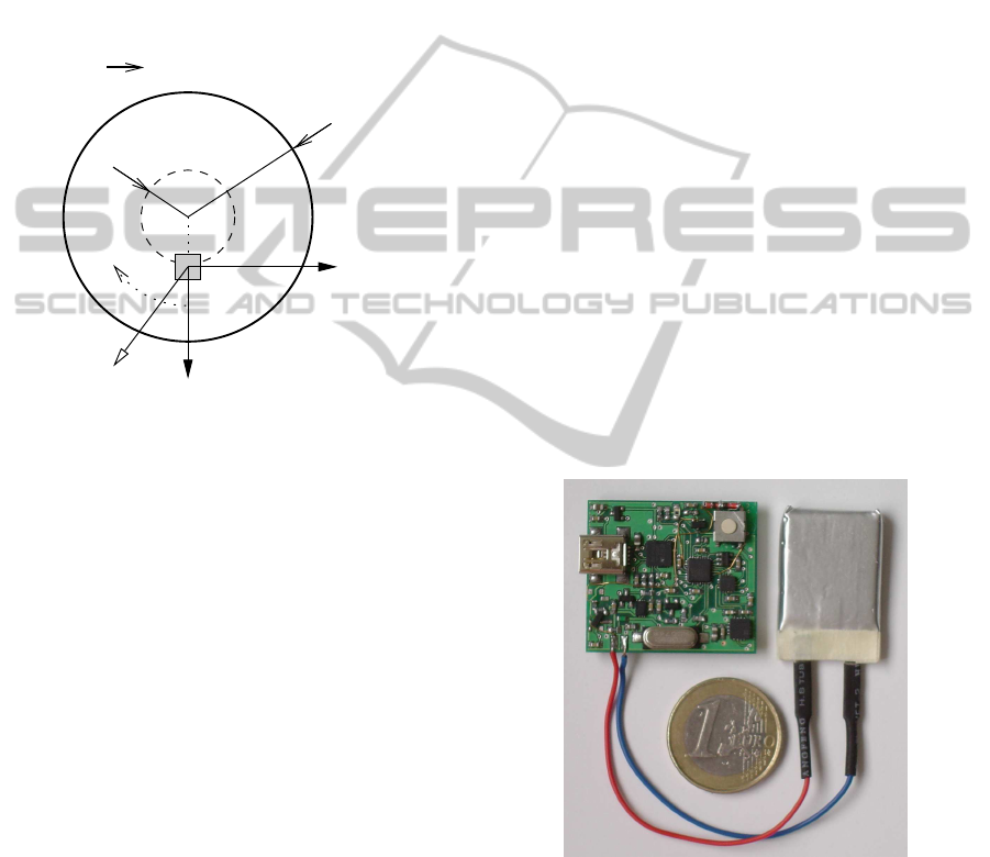
Figure 1: Sensor position for wheel angle θ=0 (grows posi-
tive in driving direction). Angular acceleration is measured
by a
1
, centrifugal force by a
2
, and the gyroscope measures
angular wheel speed ω.
An early reference to a sensor mounted on wheels
for odometry was presented in (Coulter et al., 2011)
for all kinds of wheelchairs. In (Sonenblum et al.,
2012), this sensor was validated for the measurement
of wheelchair movement as a tool for clinical experi-
ments in the area of shoulder health and to collect data
for wheelchair improvements. The sensor is mounted
on the wheel as in Figure 1 and the wheel angle is
derived from low-pass filtered a
1
and a
2
accelerome-
ters using atan2. The result is again low pass filtered
using a butterworth characteristic with a 3 Hz cut off
selected to fit the maximal wheelchair speed of 1.5
m/s (downhill) and then doubled. Based on MEMS
sensors, it records the data on an SD-card for offline
analysis. The description of hard and software for this
sensor is available in (Sonenblum, 2010). The method
inherently produces angle errors while the wheelchair
is accelerated or exposed to noise from driving over
uneven terrain. However, this method is acceptable
for hand operated wheelchairs, since the acceleration
of such vehicles is very limited, and large wheels ro-
tate slowly and suppress noise from uneven terrain
better than small wheels.
In (Huang and Wang, 2011), a similar sensor was
developed for an inertial measurement system used
on bicycles by fusing odometry with a compass as
a support for a GPS-based navigation system. The
sensor uses two accelerometers (no gyroscope) and
transmits the data via Bluetooth to an Android based
smartphone. They use a very similar approach of low
pass filters and atan2 angle computation as in (So-
nenblum et al., 2012). Due to the increased wheel
rotational speed, they observed significant accelera-
tion shifts on the a
2
accelerometer, and also on the
a
1
accelerometer (e.g. when the bicycle brakes). To
cope with centrifugal force, accelerometers were con-
figured to the maximal available range of 8 g. Offsets
from growing centrifugal forces (a
2
) or vehicle accel-
eration (a
1
) were computed by low pass filtering the
corresponding signal to subtract them from the origi-
nal signal before angle computation.
All these approaches address the sensor-fusion
problem in a rather heuristic way. Our contribution
here is to provide a principled textbook-style solution
that a) identifies how the measurements depend on the
wheel motion as the quantity to be estimated and b)
uses an Extended Kalman Filter to do the sensor fu-
sion based on the model obtained in a).
3 SENSOR HARDWARE
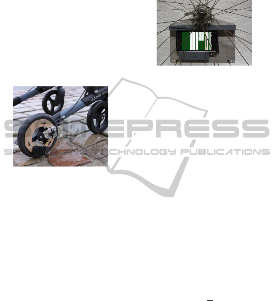
Figure 2: Prototype sensor with 3 axis accelerometer and
3-axis gyroscope used as a wheel sensor on a walker (see
Figure 3).
The experiments were conducted using two different
sensors. The prototype sensor in Figure 2, which
was mounted on a walker wheel shown in Figure 3,
uses MEMS sensors from STMicroelectronics, a 3-
axis accelerometer (MMA7361L), a 2-axis gyroscope
(LPR530AL), and a single gyroscope (LY530ALH).
Raw sensor data is sent out via Bluetooth Serial Port
AKalmanFilterforOdometryusingaWheelMountedInertialSensor
389
Profile (SSP) at a (low) frequency of ∼ 40 Hz, and
time stamped later in the receiving PC. According to
the datasheets, the limits are 6 g (g = 9.81 m/s
2
) and
1200 deg/s (20.9 rad/s), and the board reaches 4.8
g and 8.2 rad/s. Mounted on a small hard plastic
wheel with radius r
w
= 10 cm and the sensor chip at
a radius of about r
s
= 7 cm (instead of a more cen-
tered position for reduced centrifugal force), the con-
ditions for producing good results are not ideal. Al-
though the noise level is high, it is still small com-
pared to noise produced by driving on uneven terrain,
and could therefore be used for the experiments.
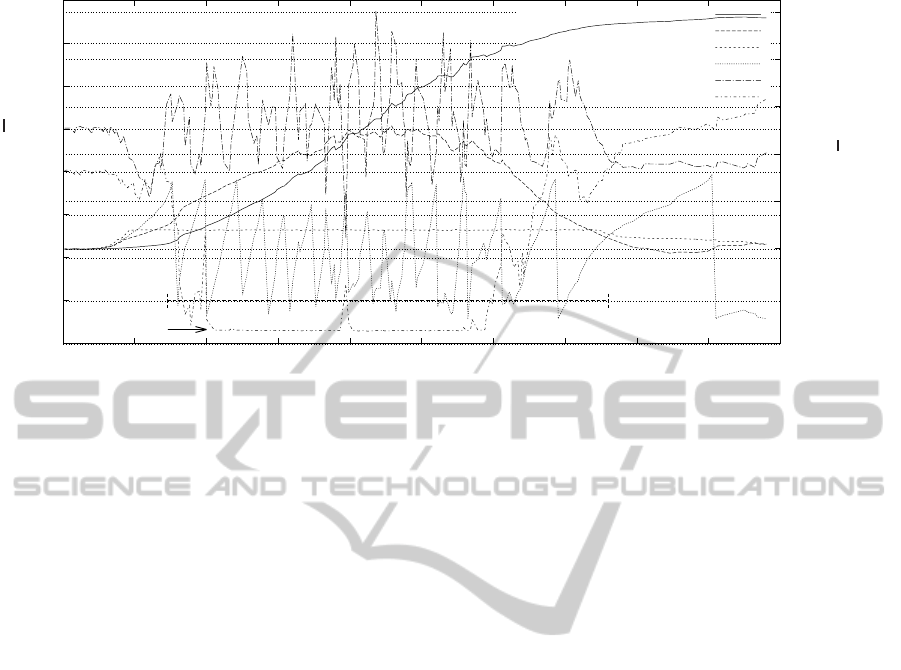
Figure 3: Prototype sensor mounted on a light-weight
walker standing on cobblestone with wireless data commu-
nication.
The second sensor is a standard smartphone (Sam-
sung Galaxy S2), mounted on a bicycle wheel hub
as shown in Figure 4 and used as a data recorder
for offline analysis. According to (Chipworks, 2011),
it contains MEMS sensors from STMicroelectronics,
a 3-axis accelerometer (LIS3DH) with limits config-
urable between 2 and 16 g, and a 3-axis gyroscope
(L3G4200D) configurable with 250, 500, or 2000
deg/s, but the Android API can only use the default
configuration of 500 deg/s and 2 g. Sensor data is re-
ceived time stamped through the API at a rate of ∼ 70
Hz. It is used here to show a reference recording un-
der optimal conditions, and for a long distance test
(Section 5.4).
4 EKF BASED SENSOR FUSION
4.1 Overview of the Extended Kalman
Filter
The Extended Kalman Filter (EKF) is a generic sen-
sor fusion algorithm for non-linear state estimation.
A very accessible introduction is given by (Welch and
Bishop, 1995) and we refer the reader to Table 2.1 and
2.2 therein for the concrete equations.
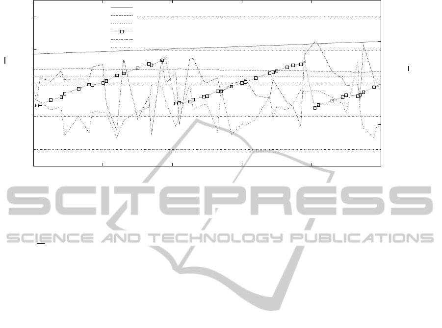
Figure 4: A Samsung Galaxy S2 as a wheel sensor at radius
r
s
= 9.5 cm in a bicycle wheel of radius r
w
= 35 cm for data
logging.
Conceptually, the EKF computes an estimate ˆx
k
for
an unknown state vector x
k
at every point in time k
from a sequence of measurement vectors z
1...k
provid-
ing noisy information about the state x
k
and optionally
control inputs u
1...k
which we don’t need here. The
point that makes the EKF attractive is that it updates
recursively an internal state representation with each
arriving z
k
(and u
k
).
This computation is based an a) a process model
f that maps a former state (optionally control input),
and noise values to a new state thereby describing,
how the state changes over time and b) a measure-
ment model h that maps state and noise values to a
measurement.
In our implementation of wheel odometry with an
EKF, the generic filter algorithm is provided by the
kfilter-library from (Zalzal, 2013), while the specific
process and measurement model are developed in the
following subsections.
4.2 State Representation
For wheel odometry the desired quantity is the posi-
tion p, i.e. the travelled horizontal distance of the ve-
hicle (measured at the center of the wheel, not at the
sensor). We drop the index
k
here for simplicity. As
we assume a non-slipping wheel, the wheel angle θ
relates linear to p as
θ =
p
r
w
(1)
with wheel radius r
w
. The sensor itself however,
makes a spiralling motion composed of a translation
by p and a rotation by θ. This complex motion leads
to the following effects (Huang and Wang, 2011) ob-
served through the sensor (Figure 1):
The gyroscope ω observes
1. Rotation, i.e. ˙p;
2. Sensor noise.
The accelerometers a
1
,a
2
observe
ICINCO2013-10thInternationalConferenceonInformaticsinControl,AutomationandRobotics
390

-15
-10
-5
0
5
10
15
0 2 4 6 8 10
0
2
4
6
angle (rad), acceleration (
m
s
2
)
distance (m), speed (
m
s
)
time (s)
(1) EKF distance
(2) EKF speed
(3) ω scaled to m/s
(4) wheel angle
(5) a
1
(6) a
2
(7) EKF acceleration
Figure 5: Measurement using the Galaxy S2 sensor (Figure 4) in a bicycle wheel shuffled indoor over a distance of 6.6 m at
walking speed.
3. Gravity;
4. Vehicle acceleration ¨p;
5. Angular acceleration in a
1
, which is proportional
to ¨p
6. Centrifugal acceleration in a
2
, which is propor-
tional to ˙p
2
;
7. Acceleration caused by uneven terrain;
8. Sensor noise.
We model the last two items as white noise. To model
the other effects as a function f of the state x, the state
x consists of
x =
p
˙p
¨p
(2)
i.e. position, velocity and acceleration.
It is common practice to include only position and
velocity in the state and model the accelerometermea-
surement as change in velocity in the control input u
(similar with the gyroscope). This is difficult here,
as from the above list of effects the relation between
measured acceleration and the state is rather complex,
so we chose also to include the acceleration ¨p in the
state.
4.3 Process Model
As usual, the process model x
k+1
= f(x
k
,w
k
) simply
integrates ¨p twice for a duration of ∆t starting from ˙p
and p. It assumes that white noise added to the accel-
eration (resulting implicitly also velocity and position
noise).
f
p
˙p
¨p
,w
=
p + ˙p∆t +
1
2
¨p∆t
2
˙p + ¨p∆t
¨p +w
(3)
The acceleration is modeled as a so-called random
walk, i.e. accumulated small random noise, which
means that the acceleration may change smoothly
over time. As usual, the noise value w is unknown, as-
sumed zero mean, independent and with known vari-
ance q = (0.07 m/s)
2
. In addition, equation (3) de-
fines that noise occurs only by this uncertain accel-
eration, since in principle every change in position
is caused by velocity and every change in velocity is
caused by acceleration.
4.4 Measurement Model
As the process model is completely driven by the
state, there is no control input u, both the accelerom-
eters and gyroscope are modeled as measurements
z. The measurement z = (a
1
,a
2
,ω)
T
consists of the
two accelerometer measurements a
1
, a
2
and the gyro-
scope measurement ω (Figure 1).
The measurement model z
k
= h(x
k
,v
k
) formalizes
the items from Section 4.2, defining how the measure-
ment z depends on the state x and the noise values v
(all at time k):
h
p
˙p
¨p
,
v
1
v
2
v
3
=
−gsinθ + ¨pcosθ − ¨p
r
s
r
w
+ v
1
−gcosθ − ¨psinθ − ˙p
2
r
s
r
2
w
+ v
2
− ˙p
1
r
w
+ v
3
(4)
AKalmanFilterforOdometryusingaWheelMountedInertialSensor
391
-40
-20
0
20
40
5 5.2 5.4 5.6 5.8 6
-10
-5
0
5
10
acceleration (
m
s
2
)
distance (m), speed (
m
s
, angle (rad)
time (s)
(1) EKF distance
(2) EKF speed
(3) ω scaled to m/s
(4) wheel angle
(5) a
1
(6) a
2
Figure 6: The sensor of figure 2 at radius r
s
= 7 cm on a walker with a wheel radius of r
w
= 10 cm. It shows 1 second with
about 2.5 wheel revolutions while driving at an extremely uncomfortable speed of 1.5 m/s on cobblestone near the limit of
the EKF filter.
where θ =
p
r
w
, r
s
is the radius of the sensor placement
on the wheel (Figure 1) and θ = 0 corresponds to the
sensor in lowest position. Equation 4 models grav-
ity (1
st
column), translational acceleration (2
nd
col-
umn), and angular as well as centrifugal acceleration
(3
rd
column) in the first two rows for the accelerom-
eter measurements a
1
and a
2
. Gravity and transla-
tional acceleration include sine and cosine terms be-
cause their direction is world-fixed but measured by a
rotating sensor. On the contrary, angular and centrifu-
gal acceleration are sensor fixed as they “rotate with
the sensor”.
The third row simply models the rotational veloc-
ity
˙
θ of the wheel as measured by the gyroscope.
All three measurements are perturbed by white
Gaussian noise v
1...3
, which is as usual unknown
and assumed independent with zero mean and vari-
ance r
1,2
= (5 m/s
2
)
2
for the accelerometer and r
3
=
(0.5 rad/s)
2
for the gyroscope. The large accelerom-
eter noise models uneven terrain.
As noted in Section 3, the gyroscopes of both
sensors do not measure rotation speeds above 10
rad/s. Therefore, a dynamic variance increased to
r
3
= (150 rad/s)
2
was used, when the gyroscope was
operated in saturation. Increasing and decreasing the
variance for r
3
smoothly increases the stability of the
filter.
Larger centrifugal forces can also lead to a satu-
ration of the a
2
accelerometer (see Section 5.2). For-
tunately, the filter continues to work under these con-
ditions, benefitting from using a dynamic variance in-
creased to r
2
= (1200m/s
2
)
2
for the a
2
measurement
to (almost) ignore this value. The variance r
2
is also
smoothly increased and reduced as for the gyroscope.
4.5 Intuitive Understanding
In this section we provide an intuitive answer to the
question Where does the distance information p come
from?
In slow motion a
1
and a
2
effectively measure
gravity only, i.e. sinθ and cosθ, while the gyro-
scope measures
˙
θ. Therefore, the overall EKF
fuses rather precise differential information (gyro-
scope) with rather imprecise absolute information
(accelerometers). Such a scenario is very common,
for instance in robot localization (Thrun et al., 2005).
With faster and more unsteady motion the situa-
tion is more difficult, as heavy accelerations strongly
perturb (a
1
,a
2
) in one dimension. However, as long
as the gyroscope is still working the filter only needs
some average information over roughly a revolution
to prevent the gyroscope errors from accumulating.
This information is available, since the integral of ¨p
is proportional to the velocity measured by the gyro-
scope.
It is more surprising that the filter still works in
fast motion and without a gyroscope (due to satura-
tion), as we will report in section 5.2. To our judge-
ment, at higher speeds the gravity acceleration has a
very periodic pattern on which the filter “locks in”,
similar to a PLL (phase-locked loop) radio receiver.
ICINCO2013-10thInternationalConferenceonInformaticsinControl,AutomationandRobotics
392
-50
-40
-30
-20
-10
0
10
20
30
0 0.5 1 1.5 2 2.5 3 3.5 4 4.5 5
0
2
4
6
8
10
acceleration
m
s
2
distance (m), speed (
m
s
), angle (rad)
time (s)
gyroscope deactivated
a
2
saturation
(1) EKF distance
(2) EKF speed
(3) ω scaled to m/s
(4) wheel angle
(5) a
1
(6) a
2
Figure 7: Measurement using the configuration from Figure 6 driving indoor on a carpet. The walker was accelerated and
stopped on a distance of 9.70 m to a maximum speed of about 4 m/s.
5 MEASUREMENTS AND
RESULTS
The filter has been implemented as a standalone C
++
program using the kfilter-library from (Zalzal, 2013)
for offline optimizations, and as a real time applica-
tion in SimRobot, a C++ framework for robotic appli-
cations (Laue and R¨ofer, 2008).
It has been tested with different hardware under
normal conditions, as well as under extreme condi-
tions to show its limits. For the intended application
area, the focus is to demonstrate the correct recogni-
tion of complete wheel revolutions. Therefore, the
rolling distance for each experiment was measured
to check the deviations of the sensor measurement,
and the obtained graphical representation was dou-
ble checked to identify the combination of missing
or false detection of wheel revolutions. The long dis-
tance test described in Section 5.4 uses an indepen-
dent sensor to count wheel revolutions.
Figure 5 shows a measurement using a bicycle
wheel with the Samsung Galaxy S2 shown in Fig-
ure 4 under optimal conditions and walking speed.
The travelled distance measured by the EKF is shown
by curve (1), the EKF speed (2) and the gyroscope
measurement (3) are almost identical (the curve at the
bottom). The rotational speed of the gyroscope was
scaled to its corresponding vehicle speed to allow a
comparison with the derived EKF speed. The wheel
angle (4) is derived from the EKF distance (normal-
ized to a range from −π to π) for the interpretation
of the sensor inputs a
1
(5) and a
2
(6), that must be
sychronous, if the filter works correct.
5.1 Uneven Terrain
The measurement of Figure 6 was taken from the
third in a series of 3 successive measurements with
increasing speed, using the lightweight walker driv-
ing on cobblestone (Figure 3) and the prototype sen-
sor (Figure 2). The walker reached a speed of 1.5
m/s
2
, which is already a very uncomfortable speed.
The same speed is mentioned in (Coulter et al., 2011)
as the maximal measured speed typically reached by
wheelchair drivers using hand propulsion. The hard
plastic wheels provide almost no damping and the
a
2
measurement contains peaks ranging from +15 to
−40 m/s
2
, which makes it even hard for a human
reader to see the sinusodial effect of gravity. The gy-
roscope was deactivated after 2 seconds (saturation)
and activated short before the target.
This experiment shows, that the filter can cope
with uneven terrain at a speed near the limit reach-
able by elderly people, but certainly far beyond a level
of comfortable driving, even with a deactivated gyro-
scope. The observable noise on the EKF distance is
significant, but would be much smaller using a gy-
roscope covering the full measurement range, as dis-
cussed in Section 5.3.
5.2 High Speed
Figure 7 uses the walker from Section 5.1 for driv-
ing in an indoor environment on a carpet over a dis-
AKalmanFilterforOdometryusingaWheelMountedInertialSensor
393

-50
-40
-30
-20
-10
0
10
20
30
40
0 0.5 1 1.5 2 2.5 3 3.5 4 4.5 5
-15
-10
-5
0
5
10
15
acceleration (
m
s
2
)
deviation (cm), speed (
m
s
)
time (s)
maximal deviation (14.5 cm)
maximal deviation with gyroscope (1.8 cm)
gyroscope deactivated
a
2
saturation
(1) ω scaled to m/s
(2) true speed
(3) EKF speed
(4) deviation (cm)
(5) with gyro (cm)
(6) a
1
(7) a
2
Figure 8: Simulated scenario based on the measured data of the scenario in Figure 7. The simulation allows the printing of
the deviation between EKF distance and true distance (4).
tance of 9.70 m. The walker was accelerated (shuf-
fled) within 2 seconds to a maximum speed above 4
m/s. The gyroscope is saturated after 0.7 s. Centrifu-
gal force reaches values of about 12 g in this exper-
iment, which saturates the a
2
accelerometer (6) after
one second. Again, the EKF derived final distance (1)
coincides with the reference measurement.
This experiment is a clear indication, that our EKF
filter can cope with high speeds and heavy accelera-
tions, even if two of the three sensors are already in
saturation. The reached speed is far beyond the speed
reachable by users dependent on a walker.
5.3 Angle Truth
Comparing the computed angle with the real angle
is desirable, but requires an independent secondary
odometry sensor, which may introduce additional un-
certainties, especially considering synchronization.
To analyse the EKF filter alone, we place it in a sim-
ulation loop based on the kinematic model used for
the filter itself, and feed the filter with (noisy) sensor
input based on a fully known state x.
Figure 8 is a simulation of the high speed sce-
nario described in Section 5.2. Here, the difference
between simulated position and the derived distance
is given as the dotted line (4) in cm. In this scenario,
the vehicle was accelerated for 1.5 s with 3.2 m/s
2
,
rolled for 0.5 s, and then braked with -3.2 m/s
2
, the
resulting simulated speed is visualized as curve (2).
The sensor data contains noise using a normal distri-
bution (Box and Muller, 1958) with a standard devia-
tion σ = (0.5+ ˙p) m/s
2
for the accelerometers (curve
(6) and (7)). The noise grew with the simulated speed
to create noise similar to noise from driving on un-
even terrain. For the gyroscope, σ = 0.5 m/s and a
linear error by multiplication with 1.01 were chosen.
The maximal difference of 14.5 cm (wheel angle er-
ror near 90 degrees) confirms this example to be an
extreme case. Although speed and acceleration where
chosen extremly high, the EKF filter did not loose a
single wheel revolution.
This experiment was repeated with the gyroscope
measuring the full range of angular speed (no gyro-
scope saturation). Curve (5) in Figure 8 is the differ-
ence for this configuration, where the maximal devia-
tion does not exceed 1.8 cm.
In this example, while driving over a distance of
9.70 m, the gyroscope would overestimate the dis-
tance due to its linear error by nearly 10 cm. The
filter corrects the gyroscope measurement using the
additional information from the a
1
accelerometer to
correct this error, reducing it to an overall maximal
difference of 1.8 cm. Using the gyroscope not only in-
creases the precision, it also suppresses underground
noise as it is mainly unaffected by vibrations.
5.4 Long Distance
For a long distance test, the bicycle sensor was used
over a distance of 4 km in an urban environment
with segments of cobblestone and typical bumps at
speeds up to 6 m/s (22 km/h). As a reference mea-
surement, a magnet was attached to the fork carrying
the wheel to count complete wheel revolutions. The
result was 1828 wheel revolutions for the magnetic
ICINCO2013-10thInternationalConferenceonInformaticsinControl,AutomationandRobotics
394

counter, 1827.6 for the EKF filter. It therefore works
correctly in a practical scenario.
6 CONCLUSIONS
This paper presents a sensor fusion algorithm for a
wheel mounted accelerometer and gyroscope based
odometry sensor. In contrast to existing approaches
using ad hoc methods to derive wheel angles, the
presented solution uses an Extended Kalman filter as
a principled estimator for locally linear systems ob-
served by noisy sensors. The power of this algo-
rithm is demonstrated by the overall positve results of
a number of experiments using real hardware under
normal as well as extreme conditions, and by simula-
tion experiments to compare the filter output against
a well known true state. The filter adapts dynamically
to saturation of the gyroscope and of the centrifugal
force accelerometer at high speed and continues to
work with even a single accelerometer. Embedded
in a small hardware component, it will provide a very
simple way of belated or temporary installation for
existing vehicles.
ACKNOWLEDGEMENTS
The author wishes to thank Hui Shi for her intensive
rereading, Christian Mandel and Christoph Budelman
for providing the prototype sensor, and Bernd Krieg-
Br¨uckner as the initiator for this work and coordinator
of the (collaborative)project ASSAM (EU AAL Joint
Programme AAL-2011-4-062, Call 4 ICT Based So-
lutions for Advancement of Older Persons’ Mobility.
REFERENCES
Bluetooth (2013). Bluetooth Specification Version 4.0.
http://www.bluetooth.org/.
Box, G. E. P. and Muller, M. E. (1958). A note on the
generation of random normal deviates. The Annals of
Mathematical Statistics, 29(2):610–611.
Chipworks (2011). Silicon Summary in the Samsung
Galaxy S II. http://www.chipworks.com/.
Coulter, E. H., Dall, P. M., Rochester, L., Hasler, J. P., and
Granat, M. H. (2011). Development and validation of
a physical activity monitor for use on a wheelchair.
Spinal Cord 2010, 49:455–50.
Huang, J.-D. and Wang, T.-W. (2011). Accelerometer based
wireless wheel rotating sensor for navigation usage. In
Sensing Technology (ICST), 2011 Fifth International
Conference on Sensing Technology, pages 565–568.
Kalman, R. E. (1960). A new approach to linear filtering
and prediction problems. Transactions of the ASME–
Journal of Basic Engineering, 82(Series D):35–45.
Krieg-Br¨uckner, B., Bothmer, H., Budelmann, C., Crombie,
D., Guerin, A., Heindorf, A., Lifante, J., Martinez, A.,
S.Millet, and Vellemann, E. (2012). Assistance for
Safe Mobility: the ASSAM Project. In Proceedings
of the AAL-Forum 2012, Eindhoven.
Krieg-Br¨uckner, B., Gersdorf, B., Mandel, C., and
Schr¨oder, M.-S. (2013). Navigation Aid for Mobility
Assistants. In Proceedings of the Joint CEWIT-TZI-
acatech Workshop “ICT meets Medicine and Health”
ICTMH 2013.
Laue, T. and R¨ofer, T. (2008). SimRobot - Development
and Applications. In Proceedings of the International
Conference on Simulation, Modeling and Program-
ming for Autonomous Robots SIMPAR 2008.
OpenStreetMap (2013). OpenStreetMap - The Map.
http://www.openstreetmap.org/.
Sonenblum, S. (2010). How to Build a Wheelchair
Data Logging System. http://www.mobilityrerc.
gatech.edu/wheelchair
data logger.php/.
Sonenblum, S. E., Sprigle, S., Caspall, J., and Lopez, R.
(2012). Validation of an accelerometer-based method
to measure the use of manual wheelchairs. Medical
Engineering Physics, 34(6):781–786.
Thrun, S., Burgard, W., and Fox, D. (2005). Probabilis-
tic Robotics (Intelligent Robotics and Autonomous
Agents). The MIT Press.
Welch, G. and Bishop, G. (1995). An introduction to the
Kalman filter. Technical Report 95-041, University of
North Carolina, Chapel Hill, NC, USA.
Zalzal, V. (2013). KFilter - Free C++ Extended Kalman
Filter Library. http://http://kalman.sourceforge.net/.
AKalmanFilterforOdometryusingaWheelMountedInertialSensor
395
