Tensor Systems

Multilinear Modeling and Applications

G. Pangalos

, A. Eichler

and G. Lichtenberg

Institute of Control Systems, Hamburg University of Technology, Eißendorfer Straße 40, Hamburg, Germany

Faculty of Life Sciences, Hamburg University of Applied Sciences, Lohbr

ugger Kirchstraße 65, Hamburg, Germany

Keywords:

Multilinear Systems, Hybrid Systems, Tensor Decomposition, Heating Systems, Multi-Agent Systems.

Abstract:

Tensor systems are a framework for modeling of multilinear hybrid systems with discrete and continuous

valued signals. Two examples from building services engineering and multi-agent systems show applications

of this framework. A tensor model of a heating system is derived and approximated by tensor decomposition

methods ﬁrst. Second, a tensor model of a multi-agent system with a structure already given in a decomposed

form is reduced further by the same decomposition methods. The validity of these low rank approximations is

shown for both examples.

1 INTRODUCTION

Multilinear models are a subclass of nonlinear mod-

els which is interesting for engineering applications

because several systems behave multilinear, as shown

by the examples. In most applications the processes

are driven by some automation device with ﬁxed sam-

pling time. Thus, only discrete time models are inves-

tigated here.

The class of multilinear models obviously in-

cludes linear continuous valued models but moreover,

all discrete valued models are inherently multilinear,

see (Lichtenberg, 2010). As multilinearity is mathe-

matically closely related to tensor calculus, there are

tensor representations of multilinear systems. Of spe-

cial interest are discrete time hybrid systems consist-

ing of a multilinear continuous valued subsystem and

an arbitrary discrete valued subsystem connected by

a quantizer and an injector. These can be represented

by so-called Hybrid Tensor Systems deﬁned in (Licht-

enberg, 2011). This modeling approach was ﬁrst ap-

plied to the identiﬁcation problem of discrete valued

models from continuous data, (Lichtenberg and Eich-

ler, 2011).

Over the last years simulation of building and

heating systems has attracted a lot of interest, see

e.g. (Nouidui et al., 2012) or (Wetter, 2006). In these

approaches nonlinear models are derived and simu-

lated, mostly for performance evaluation. Heating

systems are application examples for hybrid tensor

systems because of their physical structure, see (Pan-

galos and Lichtenberg, 2012). This paper shows in

detail how to derive a multilinear one zone model of

a large scale building using RC-models of the walls.

Another ﬁeld of applications are distributed net-

work systems like Multi-Agent Systems (MAS),

which have received considerable attention over the

past ten years, because of its broad variety of applica-

tions, see (Ren and Beard, 2007; Ren and Cao, 2011).

To perform tasks like Decision-Making or Policy For-

mulation, hybrid MASs are required, (Srinivasan and

Choy, 2010). These can be represented by the same

class of hybrid tensor systems.

Numerical tensor calculus with special interest

on decomposition methods is an active reseach ﬁeld

in applied mathematics, see e.g. (Hackbusch, 2012).

Tensor models can be approximated by standard ten-

sor decomposition techniques - similar to model re-

duction techniques for linear systems. Most of the

latter techniques like PCA use singular value decom-

postion (SVD) of matrices as workhorse for the re-

duction process. For tensor systems, so-called higher-

order SVD decomposition algorithms are appropriate

reduction methods, see (Kolda and Bader, 2009).

The paper is organized as follows. After this intro-

duction the class of hybrid tensor systems is described

in section 2. The model of a complex heating system

is developed, validated, represented by a hybrid ten-

sor system, and ﬁnally decomposed in section 3. In

section 4 multilinear modeling and transformation to

a tensor system is shown for a hybrid MAS. Final con-

clusions are drawn in section 5.

275

Pangalos G., Eichler A. and Lichtenberg G..

Tensor Systems - Multilinear Modeling and Applications.

DOI: 10.5220/0004475602750285

In Proceedings of the 3rd International Conference on Simulation and Modeling Methodologies, Technologies and Applications (SIMULTECH-2013),

pages 275-285

ISBN: 978-989-8565-69-3

 2013 SCITEPRESS (Science and Technology Publications, Lda.)

2 TENSOR SYSTEMS

Tensor representations of multilinear systems are in-

troduced in (Lichtenberg, 2011) and reviewed in this

section. All linear systems can be represented by this

class, which on the other hand is a subset of the class

of polynomial systems.

First, a matrix format to describe multilinear sys-

tems is introduced. Next, it is shown how to represent

these systems as tensor models. Finally, the notation

is extended to hybrid systems which include continu-

ous and discrete states and inputs.

2.1 Multilinear Matrix Models

With the help of the symbol ⊗ denoting the standard

Kronecker product, the monomial vector introduced

in the following Deﬁnition contains all possible mul-

tilinear terms.

Deﬁnition 2.1. The monomial vector is deﬁned as

m(x, u)=





⊗ ··· ⊗





⊗





⊗ ··· ⊗





(1)

where x ∈ R

is the state vector and u ∈ R

is the

input vector.

With the monomial vector, a multilinear state

space model can be written in matrix form

Φ(x) = F m(x, u) , (2)

y = G m(x, u) , (3)

where Φ(x) denotes the next state vector, y ∈ R

the output vector, F ∈ R

n×2

(n+m)

the transition matrix

and G ∈ R

l×2

(n+m)

the output matrix.

Example 2.1. Consider the state transition function

of a multilinear second order model with one input

and next state vector



+ f

u+ f

+ f



The state space model (2) is given as



Φ(x

)

Φ(x

)





0 0 f

0 0

0 f















(4)

In the following, the output equation (3) will not

be considered – for a description of multilinear input-

output models see (Lichtenberg, 2011).

For multilinear models (2), linear state and input

variable transformations

˜x

− b

∀i = 1, . . . , n (5)

˜u

− b

n+i

∀i = 1, . . . , m (6)

are computable in closed form. The transformed state

transition matrix is given by

F = diag

i=1,...,n







FT −



b 0

n×2

(n+m)

−1



(7)

where diag denotes the diagonal matrix with ele-

ments a

T =



1 0

n+m



⊗ ··· ⊗



1 0



is a transformation matrix, b is a column vector con-

taining the b

’s and 0

n×2

(n+m)

−1

denotes a zero ma-

trix with dimension (n × 2

(n+m)

− 1). Linear transfor-

mations allow a numerical preconditioning of models

which is used in section 3.4.

2.2 Multilinear Tensor Models

To rewrite (2) in a compact tensor notation, follow-

ing standard deﬁnitions from e.g. (Kolda and Bader,

2009) or (Cichocki et al., 2009) are introduced.

Deﬁnition 2.2. A Tensor

X ∈ R

×I

×···×I

of order n is an n-way array where elements x

···i

are indexed by i

∈ {1, 2, . . . I

} for j = 1, . . . , n.

Example 2.2. The elements of a tensor X ∈ R

2×3×2

can be illustrated and arranged in 3 dimensions as

211

221

231

111

121

131

212

222

232

112

122

132

Deﬁnition 2.3. A Kruskal tensor

K = [X

, X

, . . . , X

] · λ ∈ R

×r

×···×r

is a tensor of dimension (r

, . . . , r

), with elements

given by the sums of the outer products of the col-

umn vectors of so-called factor matrices X

∈ R

×r

weighted by the elements of the so-called weighting

or parameter vector λ. An element of the multidimen-

sional tensor K is given by

jk...p

∑

i=1

)

. . . (X

)

If no weighting vector is given, it is assumed to be

a vector of ones, i.e. λ = (1 1 . . . 1)

SIMULTECH2013-3rdInternationalConferenceonSimulationandModelingMethodologies,Technologiesand

Applications

276

Deﬁnition 2.4. The contracted product of two ten-

sors Y ∈ R

×...×I

and X ∈ R

×...×I

×I

n+1

×...×I

n+m

, . . . , k

) =

∑

···

∑

,...,i

,...,k

,...,i

(8)

is a tensor of dimension I

n+1

× . . . × I

n+m

Example 2.3. Consider a tensor X ∈ R

2×2×3

and a tensor Y ∈ R

2×2

. To calculate the con-

tracted product Z =

∈ R

, the matching

dimensions have to be multiplied elementwise, as

highlighted in red in the following illustrations.

211

221

111

121

212

222

112

122

213

223

113

123

211

221

111

121

212

222

112

122

213

223

113

123

211

221

111

121

212

222

112

122

213

223

113

123

A simple notation for tensor spaces is introduced:

(n+m)

:= R

n+m

z}|{

2×...×2

The state transition function (2) of a multilin-

ear state space model can then be rewritten with the

monomial Kruskal tensor

M(x, u) =





, . . . ,









, . . . ,





in terms of a contracted tensor product as

Φ(x) =

M(x, u)

, (9)

where the transition tensor F ∈ R

(n+m)

2×n

contains all

parameters of the model while the structure is given

by the monomial tensor M(x, u) ∈ R

(n+m)

2.3 Decomposed Tensor Models

As contracted products could be efﬁciently computed

in Kruskal form, and monomial tensors are easily

given in this form by their internal structure, it is

worth looking for decompositions

F = [F

, . . . , F

, F

, . . . , F

, F

] · λ

(10)

of the state transition tensor having r

factors. This

will be illustrated by the Example 2.1. Setting the

matrix factors of (10) accordingly leads to



1 0 1 0 0 1 0 0 1 0

0 1 0 1 1 0 1 1 0 1





1 1 1 1 1 0 0 1 0 0

0 0 0 0 0 1 1 0 1 1





1 1 0 0 1 1 1 0 0 0

0 0 1 1 0 0 0 1 1 1





1 1 1 1 0 0 0 0 0 0

0 0 0 0 1 1 1 1 1 1



Together with the continuous valued parameter vector





they form the state transition tensor

F = [F

, F

] · λ

The contracted product can now be calculated by sim-

ple matrix operations (Lichtenberg, 2011)

M(x, u)

= (11)













where ~ denotes the (element-wise) Hadamard prod-

uct. It can be checked that calculating the contracted

product (9) leads to the transition equation (4).

At a ﬁrst glance, for Example 2.1 this tensor nota-

tion does not seem to be more compact than the ma-

trix notation. It is easy to verify that the system matrix

has n ·2

(m+n)

= 16 elements, whereas the tensor repre-

sentation takes r

(1 + 3n + 2m) = 90 elements as the

dimension of the n + m factor matrices is 2 × r

, F

has dimension n ×r

and the parameter vector has an-

other r

entries.

But looking at the model of the heating system

that will be introduced in section 3 with n = 12 states,

no inputs m = 0 and r

= 46 factors, this would lead

to 12 · 2

= 49152 elements in matrix representation

whereas only 46(1 + 3 · 12) = 1702 Kruskal tensor el-

ements need to be stored.

For construction of the factor matrices and the pa-

rameter vector set the columns of the factor matrices





, if the summand contains the corresponding

state and to





otherwise. The product of states is

weighted by a constant given in the parameter vector.

The factor matrix F

indicates to which next state el-

ement the summand is added.

TensorSystems-MultilinearModelingandApplications

277

This can is shown exemplarily by the ﬁrst sum-

mand of the Example. All ﬁrst rows of the factor ma-

trices are





, i.e. the ﬁrst summand of the ﬁrst next

state does not depend on any current state or input but

is equal to the ﬁrst entry f

of the parameter vector.

With standard tensor decomposition algorithms

like CP-ALS low rank approximations of the state

transition tensor could be found, see (Kolda and

Bader, 2009).

2.4 Boolean Tensor Models

In the following, Boolean variables will be indicated

by underlining. Heading for tensor models of hybrid

systems, the binary state x ∈ B

and input u ∈ B

are

deﬁned. The state transition function of a Boolean

tensor state space model

Φ(x) =

L(x, u)

, (12)

with a transition tensor F ∈ B

(N+M)

2×N

describes a

binary dynamical system by a contracted product with

a Boolean literal tensor L(x, u) ∈ B

(N+M)

deﬁned as

L(x, u) =



¯u



, · · · ,



¯u





¯x



, · · · ,



¯x



(13)

where the bar symbol is used to denote the negation

of a variable.

If the values of the state and input variables are

from a continuous domain but the transition tensor is

still Boolean, the resulting next state is in general a

continuous variable.

With the help of the symbol

deﬁning a

contracted real tensor product which converts any

Boolean FALSE to a real zero and a Boolean TRUE to a

real one, the state transition of an algebraic Boolean

tensor state space model

Φ(x) =

L(x, u)

, (14)

can be deﬁned, where

L(x, u) =



1 − u



, · · · ,



1 − u





1 − x



, · · · ,



1 − x



. (15)

It has the property that - if all initial states and inputs

are Boolean - the state and output trajectories only

take values 0 and 1 and thus, show a behavior which

includes the behavior of the binary system.

Transformation of (14) to monomial form is pos-

sible and given by

Φ(x) =

M(x, u)

, (16)

with the transition tensor F ∈ Z

(n+m)

×n

having inte-

ger elements which are easy computable from F .

2.5 Hybrid Tensor Models

Figure 1 shows a block diagram of the class of hybrid

systems investigated further. The outputs are omitted,

it is assumed that the states can be measured.

Multilinear System

Quantizer

Binary System

Injector

Figure 1: Block diagram of a multilinear hybrid system.

Without loss of generality, it is assumed that all

discrete signals are encoded Boolean. The contin-

uous valued subsystem and the discrete valued sub-

system are connected via a quantizer and an injector

given in the next Deﬁnitions, see (Lichtenberg, 2011),

where H is a hybrid space. The hybrid state and input

vectors





∈ R

× B

(17)





∈ R

× B

(18)

are given by appending the Boolean signal vectors to

the continuous signal vectors.

Deﬁnition 2.5. The standard injector is the func-

tion α : H

×···×I

→ R

×···×I

, which is given for all

elements with index vector i ∈ N

(α(x

))







1 ∈ R if x

= TRUE ,

0 ∈ R if x

= FALSE ,

if x

∈ R .

(19)

Deﬁnition 2.6. The standard quantizer is the func-

tion β : R

×···×I

→ B

×···×I

, which is given for all

elements with index vector i ∈ N

(β(x

))

= σ(x

−

) , (20)

where the Heaviside function is given as

σ(x) =



1 if x ≥ 0 ,

0 otherwise .

(21)

These deﬁnitions make the need of explicite equa-

tions for w, w, v and v obsolete, as they can be cal-

culated with the help of the standard injector and

SIMULTECH2013-3rdInternationalConferenceonSimulationandModelingMethodologies,Technologiesand

Applications

278

the standard quantizer which are also used for the

next Deﬁnition - an extension of the contracted ten-

sor product taking into account Boolean as well as

continuous values.

Deﬁnition 2.7 (Hybrid Contracted Tensor Product).

The notation



for the hybrid contracted tensor

product implies that all values are mapped to the cor-

rect domains given by the domain of the tensor on the

left side of the contracted product



α(M(β(x)))

(22)

with standard quantizer and injector.

If the tensor on the left side has hybrid domains,

quantization and injection are applied to compute the

results corresponding to the domain on the left hand

side.

By using this Deﬁnition, the state transition func-

tion of a hybrid tensor system can be written in a very

compact way as

Φ(x

) =





, u

)





. (23)

This will be illustrated by Examples in the following

sections.

3 HEATING SYSTEMS EXAMPLE

The heating system mentioned in the introduction will

now be modeled as a hybrid tensor system. This is

possible because of the inherit multilinear nature of

heating systems.

The heating system consists of a boiler with

burner, a consumer, where a building temperature can

be measured and a pump, which is controlled (see

Figure 2)

Boiler

Burner

Consumer

Pump

Figure 2: Heating system.

Signals being real or Boolean will be clear from

the context, therefore no underlines or ”undertildes”

will be used in this section.

For each of the elements of the heating system,

ﬁrst the thermal balances are stated and then trans-

formed. After a validation of the model the factor

matrices and parameter vector are given such that the

system can be represented as a tensor system.

3.1 Differential Equations

The continuous valued states of the system are the

supply temperature T

, the return temperature T

and

the buildings temperature T

. Day oscillation and year

oscillation of the ambient temperature are modeled

by four continuous valued states T

. . . T

, two for

each oscillation. Two Boolean states X

and X

deter-

mine whether or not the buildings temperature is in

the interval where the thermostatic valves are linear,

in the lower or in the upper saturation. Two further

Boolean states H

and H

determine a supply temper-

ature above an upper limit or below a lower limit and

a Boolean state U that states if the boiler is running or

not. The state vector is given by x ∈ R

× B

x = [T

(24)

Controlled Pump

The ﬂow rate

V is a consequence of the room tempera-

ture T

and the reference temperature for the room T

The relationship is shown in Figure 3.

− T

−∆T

∆T





Figure 3: Flow rate over control error of the room tempera-

ture.

In this Figure

is the mean ﬂow rate for T

= T

and

is the amplitude from the mean ﬂow rate at ref-

erence room temperature to its extrema. The extrema

in the ﬂow rate are reached at a room temperature that

is at least ∆T

different from the reference room tem-

perature.

To state the ﬂow rate

V in terms of the discrete

states and the room temperature, the discrete states



1 if T

> T

− ∆T

0 else

(25)



1 if T

> T

+ ∆T

0 else

(26)

are introduced. Thus the ﬂow rate

V is given as

V =



∆T

−



. . .

−



∆T



−

∆T

. . .

TensorSystems-MultilinearModelingandApplications

279

∆T

. (27)

Boiler

The thermal balance of the boiler is given as

ρc = T

V ρc − T

V ρc + P

max

U . (28)

Using the Euler forward method with sampling time t

to discretize this differential equation and rearranging

leads to

(k + 1) = T

(k) −

(k)

V (k). . . (29)

(k)

V (k) +

ρc

max

U(k) .

Dropping the time index, denoting the next state by

the operator Φ and substituting (27) for the ﬂow rate

gives

Φ(T

) = T



1 −

(

)



+ T

(

)

. . .

(∆T

−T

)

∆T

− T

(∆T

−T

)

∆T

. . .

∆T

− T

∆T

. . . (30)

(∆T

)

∆T

− T

(∆T

)

∆T

. . .

−T

∆T

+ T

∆T

+ P

max

cρ

Ambient Temperature

The ambient temperature is modeled as an oscillator

with two frequencies. One for the temperature oscil-

lation over the day and one for the oscillation of the

year. The sinusoidal curves estimate the ambient tem-

perature roughly.

The continuous time state space model can be

given by



















0 1 0 0

−ω

0 0 0

0 0 0 1

0 0 −ω





















1 0 1 0















+ T

a,m

. (31)

Note that a multilinear state space model allows a

constant term, here T

a,m

. Using the Euler forward

method, the state equation in discrete time with sam-

pling time t

is given by































1 t

0 0

−ω

1 0 0

0 0 1 t

0 0 −ω



















(32)

The output equation of system (31) does not change.

Building

The temperature of the building T

is introduced as the

average temperature of all rooms. The temperature

can be given as

= k

r,b

− T

) − k

b,a

− T

) , (33)

where k

is the capacity of the building, k

r,b

the heat

transfer coefﬁcient from the radiators to the building

and k

b,a

the heat transfer coefﬁcient from the building

to the outside. Again using the Euler forward method

for temporal discretization and substituting the output

equation of (31) gives

Φ(T

) = T



1 −

r,b

b,a

)



+ T

r,b

. . .

b,a

+ T

b,a

a,m

. (34)

The parameters k

, k

r,b

, k

b,a

are estimated with real

measurement data of the building. The validation of

the model is described in the next section, where the

numerical values of the constants are given in Table 3.

Consumer

The thermal balance of the consumer is given by

(t)V

ρc = T

(t)

V (t)ρc − T

(t)

V (t)ρc −

(t) .

(35)

The heat demand

can be calculated in terms of

the return temperature and the building temperature

(t) = (T

(t) − T

(t))k

r,b

. (36)

Inserting (36) and (27) into (35) and discretizing

the result gives

Φ(T

) = T

(

)

. . . (37)

+ T



1 −

r,b

+ c

ρ + c

ρ)

cρ



. . .

+ T

r,b

cρ

− T

(∆T

− T

)

∆T

. . .

+ T

(∆T

− T

)

∆T

− T

∆T

. . .

+ T

∆T

− T

(∆T

+ T

)

∆T

. . .

+ T

(∆T

+ T

)

∆T

+ T

∆T

. . .

− T

∆T

where the time dependencies are dropped.

SIMULTECH2013-3rdInternationalConferenceonSimulationandModelingMethodologies,Technologiesand

Applications

280

Bang Bang Controller

The discrete states H

and H

are used to determine

whether or not the supply temperature T

is below

a lower limit, here: 75

◦

C or above an upper limit,

here: 95

◦

C. The signal U steering the boiler is then

computed by

Φ(U ) =







U if 75

◦

C < T

< 95

◦

1 if T

≤ 75

◦

0 if T

≥ 95

◦

. (38)

3.2 Validation of the Consumer

In this section the validation of the consumer is

shown. For this purpose the discrete bang bang con-

troller is replaced by a PI-controller as in the real

building. The ambient temperature is modeled sep-

arately. For the validation, the ambient temperature

is taken from measurement data. Not all states are

displayed but just the supply temperature T

, the re-

turn temperature T

and the ﬂow rate

V . Note that

the ﬂow rate is not a state of the system but depends

on the buildings temperature T

and the two Boolean

states X

and X

. The system has two main time scales

caused by the oscillating ambient temperature over

the day and over the year.

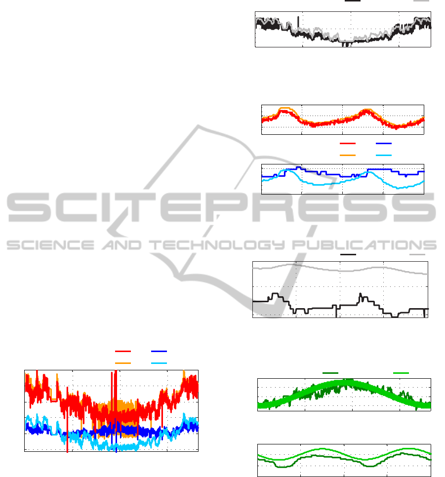
The temperatures over a whole year, starting Jan-

uary 1

are given in Figure 4. The mismatch in the

return temperature in the summer is probably caused

by a later detected bypass of the boiler.

0 100 200 300

Time [days]

Temperature [°C]

Measurement:

Simulation:

Figure 4: Supply and return temperatures over a year.

The ﬂow rate over the year is given in Figure 5.

This shows a quite good ﬁt of the signals in a year

scale. Now the second scale should be investigated.

Therefore in Figure 6 the temperatures are given and

in Figure 7 the ﬂow rate is given for two days. As

one can see also the day scale has a good ﬁt. Still

remaining for validation is the use of an oscillator for

the ambient temperature. Figure 8 shows the ambient

temperature from measurements and the results from

the oscillator over a year in the upper plot and the

0 100 200 300

x 10

−3

Time [days]

Flow rate [m

/s]

Measurement: Simulation:

Figure 5: Flow rates over a year.

Temperature

103 103.5 104 104.5 105

Time [days]

[°C]

Measurement:

Simulation:

Figure 6: Supply and return temperatures over two days.

103 103.5 104 104.5 105

x 10

−3

Time [days]

Flow rate [m

/s]

Measurement: Simulation:

Figure 7: Flow rates over two days.

0 100 200 300

Time [days]

103 103.5 104 104.5 105

Time [days]

Ambient temperature [°C]

Measurement Simulation

Figure 8: Measurement and simulation of the ambient tem-

perature.

ambient temperatures over two days in the lower plot.

The parameters for the signal generator are given in

Table 1

For completeness Table 2 states the used material

constants and Table 3 states all estimated parameters.

TensorSystems-MultilinearModelingandApplications

281

Table 1: Parameters of the ambient temperature signal gen-

erator.

Frequency Symbol Value

Day oscillation ω

−



2π

86400



rad

Year oscillation ω

−



2π

31536000



rad

Table 2: Material constants of water.

Density of water ρ 1000

Speciﬁc heat

4182

W s

Kg K

capacity of water

Table 3: Parameters of the building model.

Parameter Symbol Value

Volume boiler V

1.05m

Volume consumer V v 5m

Mean ﬂow rate

4.75 · 10

−3

Flow rate amplitude

3.25 · 10

−3

Building reference

◦

temperature

Linear temperature

∆T

◦

Camplitude of

the thermostat

Thermal capacity

W s

of the building

Total heat transfer

r,b

2.5 · 10

coefﬁcient

(radiator building)

Total heat transfer

b,a

4.7338 · 10

coefﬁcient

(building ambiance)

Mean ambient

a,m

12.5

◦

temperature

Maximal power

max

1.1MW

of the boiler

The initial state vector used is

x(0) =



253 323 294 0 −

5π

86400

. . .

−

5π

86400

− 12.5 0 1 0 0 0 1



. (39)

Note that the simulation was performed with SI-units,

such that the temperatures are in Kelvin. For bet-

ter legibility the temperatures in Table 3 were given

◦

3.3 System Tensor

With the difference equations from the section 3.1 it

is now straight forward to construct the system ten-

sor. Here just the ﬁrst entries of the system tensors

factor matrices, that correspond to the next state of

the supply temperature T

are given. The entries are

constructed as shown in Example 2.1 The Factor ma-

trices, in order of the states (24) are:



0 1 0 1 0 . . .

1 0 1 0 1 . . .



, F



1 0 1 0 1 . . .

0 1 0 1 0 . . .





1 1 1 1 0 . . .

0 0 0 0 1 . . .



, F



1 1 1 1 1 . . .

0 0 0 0 0 . . .





1 1 1 1 1 . . .

0 0 0 0 0 . . .



, F



1 1 1 1 1 . . .

0 0 0 0 0 . . .





1 1 1 1 1 . . .

0 0 0 0 0 . . .



, F



1 1 0 0 0 . . .

0 0 1 1 1 . . .





1 1 1 1 1 . . .

0 0 0 0 0 . . .



, F



1 1 1 1 1 . . .

0 0 0 0 0 . . .





1 1 1 1 1 . . .

0 0 0 0 0 . . .



, F



1 1 1 1 1 . . .

0 0 0 0 0 . . .









1 1 1 1 1 . . .

0 0 0 0 0 . . .







(40)

The matrix F

has dimension 12 × 46 to assign

the 46 summands of the system to the corresponding

next state. Note, that the factor matrices are not com-

plete but just given for the ﬁrst ﬁve summands of the

ﬁrst next state. Since all entries that were looked at

correspond to the ﬁrst next state, the ﬁrst ﬁve entries

of the ﬁrst row of F

are 1. The corresponding part

of the parameter vector is given by







1 −

(

)

(

)

(∆T

−T

)

∆T

−

(∆T

−T

)

∆T







. (41)

3.4 Tensor Decomposition

In this section a reduction of the tensor rank is per-

formed using tensor decomposition techniques. With

the factor matrices (40) and the parameter vector (41)

deﬁned in section 3 a state transition tensor

F =



, F

, . . . (42)

, F



· λ

(43)

is constructed. The Tensor Toolbox (Bader and

Kolda, 2012) and the command cp

als is used to re-

duce the rank of the tensor F, which was constructed

SIMULTECH2013-3rdInternationalConferenceonSimulationandModelingMethodologies,Technologiesand

Applications

282

to have a tensor rank of 46. Using the Toolbox, the

rank of the system tensor is reduced to 23, which has

a ﬁt of over 99%. The ﬁrst ﬁve entries of the ﬁrst two

factor matrices are



−0.999 0.999 1.000 1.000 1.000 . . .

0.045 −0.054 0.009 0.007 0.000 . . .





0.988 0.984 0.999 1.000 1.000 . . .

−0.152 −0.179 0.040 0.031 0.000 . . .



.(44)

The corresponding entries in the parameter vector are

λ =



10.443 6.967 4.322 2.598 2.587 . . .



(45)

The results of the simulation with the original and the

decomposed state transition tensor are given in Fig-

ure 9. One can see, that the main system dynamics

are captured with the decomposed system. The sup-

ply temperature drops to 75

◦

C if 95

◦

C is reached and

rises again. Also the offset and the dynamics of the re-

turn temperature show similar behavior for both state

transition functions.

0 5 10 15 20

100

Temperature [°C]

Original system

0 5 10 15 20

100

Time [hours]

Temperature [°C]

Decomposed system

Figure 9: Original and decomposed system.

The value of the states has a big impact on the

results. For this reason a state transformation (see

section 2) was performed such that all states of

the transformed system are in the interval [0 0.5].

Since we have a 12

order system a very small

factor in front of the multiplication of all states

(which was not used, i.e. 0 in the original sys-

tem) can give a next state many orders of magni-

tude away from the original next state. This ef-

fect can be reduced signiﬁcantly by normalizing the

states to the interval [0 0.5]. To illustrate this is-

sue assume, that T

= T

= 300. To calculate the

next state of T

the multiplication of all three temper-

atures is not used, i.e. Φ(T

) = . . . + 0 · T

+ . . ..

Assume a CP decompostion is performed and the

factor is now 0.001. This still gives a very good

ﬁt for the tensor. The next state of T

however

is 300

· 0.001 = 27 · 10

different to that of the orig-

inal system. In contrast to that consider a trans-

formed system. Now the states are transformed.

They are assumed to be in the interval [280 300]

and therefore transformed with

x =

x−280

leading

to T

= T

= 0.5. Again calculating the error of

the next state gives 0.5

· 0.001 = 125 · 10

−6

trans-

forming this error back to the original coordinates

gives an error of 5 · 10

−3

4 MULTI-AGENT SYSTEMS

EXAMPLE

A MAS consists of a group of agents (e.g. vehicles

with their computing entities) that exchange informa-

tion and share knowledge to solve a common task like

in (Balaji and Srinivasan, 2010). The demand of au-

tonomous MAS’s with the ability to perform tasks as

Decision-Making or Policy Formulation leads to hy-

brid MAS’s. There are various different applications

of hybrid MAS’s and many different ways to describe

them, e. g. (Srinivasan and Choy, 2010). How a hy-

brid MAS is modeled as tensor system is shown in the

following.

Graphs are a natural way to describe the com-

munication topology between agents of an MAS,

see (Mesbahi and Egerstedt, 2010). A directed

Graph G(V , E) consists of a set of N ver-

tices, representing the single agents, and a set of

edges E ⊆ V × V , describing the communication

topology. If agent i receives information from

agent k, there is an edge (k, i) ∈ E. The mainly

used matrix representation of graphs for MAS is the

Laplacian L. The normalized Laplacian is deﬁned

as (Ren and Beard, 2007)







1 if i = k and |N

| 6= 0

−

if k ∈ N

0 otherwise.

(46)

Here N

is the set of neighbors of agent i, that is de-

ﬁned as N

= {k|(k, i) ∈ E}, and |N

| is its cardinality.

Consider a MAS of N equal agents, where each

agent i = 1 . . . N is described by the switched system

Φ(x

) = ax

+ u

if Φ

−1

) ≥ 0.5

Φ(x

) = bx

+ u

if Φ

−1

) < 0.5 , (47)

with x

, u

∈ R being continuous signals

and Φ

−1

) = x

(k − 1) denoting the previous state.

By introducing the discrete signal z

= β(Φ

−1

)),

TensorSystems-MultilinearModelingandApplications

283

being the quantized state variable, system (47) can be

written as the multilinear system

Φ(x

) = (a − b)z

+ bx

+ u

. (48)

This can be described as a tensor system for one

agent i by

Φ(x





(x, z, u)





, F





(x, z, u)



(49)

with F



1 0

0 1



, F



b 1

a − b 0



, F



0 1

1 0



The control input is determined by the communi-

cation topology as u = −Lx like simple consensus

algorithms propose (Mesbahi and Egerstedt, 2010)

with x = (x

. . . x

)

, u and z deﬁned respectively.

The discrete system is easily described by

Φ(z) = β(x). (50)

The continuous part can be described as a continuous

tensor system of the form Φ(x) =





(x, z)



. It

is obvious that the continuous system only contains

multilinear terms of the form x

introduced by the

system equations of the single agents in (48), whereas

the control input is linear in x. Thus the standard

monomial tensor of dimension R

is very sparse.

A special formation monomial tensor is introduced

here as M

(x, z) ∈ H

2×2×N

(x, z) =



1 . . . 1





1 . . . 1



, I



(51)

This is a tensor of rank N in contrast to the standard

monomial tensor of rank 1.

With (51) a state transition function of a hybrid

tensor system for the overall system, with state vec-

tor x

= (x, z)

is deﬁned as

Φ(x

) =





(x, z)





(52)

with F



, F



∈ R

2×2×N×2N

. The state

transition tensor F

has the factor matrices with 2N

factors



0 0 I





−L I









a − b







. (53)

The factor matrix F

speciﬁes the state, x

= (x, z

)

First the continuous state vector x is considered. Due

to the identity matrices in F

and F

, the ﬁrst N

columns of the factor matrices describes the internal

dynamics of the agents. This can be easily seen by

comparing the ﬁrst N columns of F

and F

with F

and F

in (49). The Laplacian in F

describes the

communication between the different agents. The

fact, that the communication is linear in the states x

explains the second N vectors in F

and F

since

















= x

The discrete signal z is simply calculated

by Φ(z) = β(x), which explains the choice of

the last N columns in F

and F

Next, a hybrid tensor system with N = 100 agents

is modeled. The considered connected graph is di-

rected and contains 473 random edges. The internal

dynamics of the single agents is described by (48)

with a = 0.5 and b = 1. The number of factors of

the exact system tensor is 300 = 3N. CP decompo-

sitions of the system tensor from rank 1 to 299 have

been calculated with cp als.

0 100 200 300

Tensor norm error

Rank

Figure 10: Frobenius norm of error.

0 0.05 0.1 0.15 0.2

0.5

Continuous state

signals

Discrete time steps

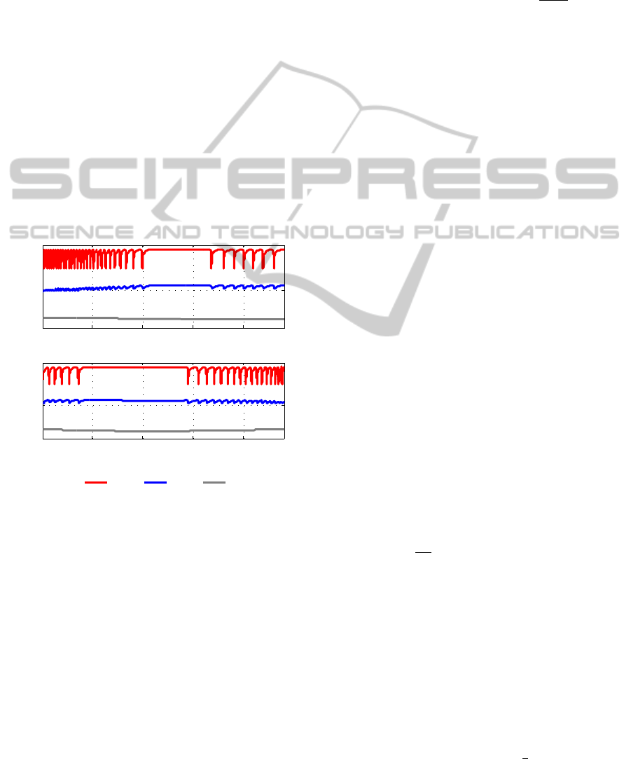
Figure 11: Continuous valued state trajectories for rank 200

approximation.

The Frobenius error between the exact and ap-

proximated hybrid tensor model is shown for tensor

approximations of different rank in Figure 10. A ten-

sor of rank 200 = 2N describes the system dynam-

ics almost exactly. The Frobenius error for graphs

of every tested different size shows qualitatively the

same shape. Thus it can be supposed that the sys-

tem is in fact not a tensor system of rank 3N but

of 2N. In Figure 11, continuous state trajectories of

the rank 200 approximation are shown. The maximal

mean squared error between the original and approx-

imated trajectories for a rank 200 approximation is

SIMULTECH2013-3rdInternationalConferenceonSimulationandModelingMethodologies,Technologiesand

Applications

284

0 0.05 0.1 0.15 0.2

0.5

Continuous state

signals

Discrete time steps

Figure 12: Continuous valued state trajectories for rank 150

approximation.

with < 10

−17

negligible and thus approximation and

original system match exactly. For comparison the

rank 150 approximation is shown on Figure 12. Here

the same consensus value of approximately 0.2 is

reached with the same convergence shape. However,

the states does not exactly converge to the real consen-

sus value but reach an envelope around it, which gets

small for higher order approximations. For approxi-

mations with smaller order instability of the conver-

gence process may occur.

5 CONCLUSIONS

Hybrid tensor systems are an adequate framework for

modeling discrete time multilinear systems with con-

tinuous and discrete valued states and inputs. A hy-

brid tensor model of a complex heating system is de-

rived as a real-world example. All parameters are

stored in a state transition tensor which in a second

step is reduced to a low rank Kruskal tensor using

standard decomposition techniques. As simulations

show, this decomposed tensor is still capable to cap-

ture the main dynamics of the heating system.

As a second application example from a quite dif-

ferent application domain, a hybrid tensor model of a

Multi-Agent System (MAS) is built. Structural con-

traints are imposed in an easy way, a reduced rank

state transition tensor of the system is again computed

by tensor decomposition algorithms and simulations

are carried out based on the decomposed model. The

reduced rank model converges to the same ﬁnal values

as the original one. Moreover, the original N-agents

system can be modeled exactly by a hybrid tensor sys-

tem with a small rank of 2N.

Further research will be done to investigate the

stability behaviour of hybrid tensor systems. Another

focus will be the derivation of tensor representations

for nonlinear normal forms - as well for general non-

linear as for multilinear systems. Tensor decompo-

sition techniques will play an important role in these

ﬁelds and extensions of the continuous algorithms to

hybrid spaces would be essential tools for analysis

and design of multilinear hybrid systems.

ACKNOWLEDGEMENTS

This work was partly supported by the project ModQS

of the Federal Ministry of Economics and Technol-

ogy, Germany.

REFERENCES

Bader, B. and Kolda, T. (2012). MATLAB Tensor Toolbox

Version 2.5. Available online.

Balaji, P. and Srinivasan, D. (2010). An Introduction

to Multi-Agent Systems, volume 310 of Studies in

Computational Intelligence, chapter 1, pages 1–27.

Springer.

Cichocki, A., Zdunek, R., Phan, A., and Amari, S. (2009).

Nonnegative Matrix and Tensor Factorizations. Wi-

ley, Chichester.

Hackbusch, W. (2012). Tensor Spaces and Numerical Ten-

sor Calculus, volume 42 of Springer Series in Com-

putational Mathematics. Springer-Verlag Berlin Hei-

delberg.

Kolda, T. and Bader, B. (2009). Tensor Decompositions and

Applications. SIAM Review, 51(3):455–500.

Lichtenberg, G. (2010). Tensor Representation of Boolean

Functions and Zhegalkin Polynomials. In Interna-

tional Workshop on Tensor Decompositions.

Lichtenberg, G. (2011). Hybrid Tensor Systems. Habilita-

tion, Hamburg University of Technology.

Lichtenberg, G. and Eichler, A. (2011). Multilinear Al-

gebraic Boolean Modelling with Tensor Decomposi-

tions Techniques. In 18th IFAC World Congress, page

TuC01.2.

Mesbahi, M. and Egerstedt, M. (2010). Graph Theoretic

Methods for Multiagent Networks. Princeton Univer-

sity Press.

Nouidui, T.S., Zuo, K.P.W., and Wetter, M. (2012). Valida-

tion and Application of the Room Model of the Mod-

elica Buildings Library. 9th International Modelica

Conference, pages 727–736.

Pangalos, G. and Lichtenberg, G. (2012). Approach to

Boolean Controller Design by Algebraic Relaxation

for Heating Systems. In 4th IFAC Conference on Anal-

ysis and Design of Hybrid Systems.

Ren, W. and Beard, R. (2007). Distributed Consensus in

Multi-Vehicle Cooperative Control - Theory and Ap-

plications. Communications and Control Engineering.

Springer Publishing Company, Incorporated.

Ren, W. and Cao, Y. (2011). Distributed Coordination of

Multi-agent Networks. Springer-Verlag London Lim-

ited.

Srinivasan, D. and Choy, M. (2010). Hybrid Multi-Agent

Systems, volume 310 of Studies in Computational In-

telligence, chapter 2, pages 29–42. Springer.

Wetter, M. (2006). Multizone Building Model for Thermal

Building Simulation in Modelica. 5th International

Modelica Conference, pages 517–526.

TensorSystems-MultilinearModelingandApplications

285