Speed Control of Drive Unit in Four-rotor Flying Robot
Stanisław Gardecki, Wojciech Giernacki and Jarosław Gośliński
Institute of Control and Information Engineering, Poznan University of Technology, 3a Piotrowo St., Poznan, Poland
Keywords: UAV, Four-rotor Flying Robot, Speed Control of Drive Unit, Coefficient Diagram Method.
Abstract: In this paper the synthesis of speed controller for drive unit is presented. Its aim is to generate the lift force
of multi-rotor flying robot. Parameters of drive unit model were experimentally determined based on
recorded time characteristics from engine test stand. The use of two alternative controllers: CDM and PID
types was proposed. The CDM controller was tuned in accordance with the Coefficient Diagram Method
and the PID controller in MATLAB’s Simulink Response Optimization tool. The efficiency of both types
control systems was compared for specified conditions. Integral quality indices were adopted as a measure
of assessment. Obtained simulation results were discussed in the context of implementation on a real robot.
1 INTRODUCTION
Many concepts of unmanned aerial vehicles have
been already developed. Usually these robots are
used in tasks of observation, patrolling and
recognition in areas of military and civil (Gertler,
2012), as well as in the science and entertainment
(Augugliaro et al., 2010). The use of several drive
units, often embedded in the same plane, is their
similarity. Such a solution (without the control of
angle of blades attack as it is in helicopters) results
with the stiff construction of whole robot, but it
enforces a specific control – change of the robot's
position and movement is only an effect of the speed
change of appropriate drive unit (DU) - obtained
from the onboard microcontroller, which aim is to
split the thrust into particular drives. A thinking
oriented to obtainment of the simplest possible
mechanical construction supported with advanced
computational unit and onboard sensors, works well
in four-rotor flying robots, but only with effective
control techniques (Gardecki and Kasiński, 2012).
In this paper, attention was focused on the
synthesis of variable speed control of one DU
(described in detail in Gardecki and Kasiński, 2012)
with the brushless DC motor and by the not well
known algorithm of the Coefficient Diagram
Method (CDM) (Manabe, 1998), which has been
already applied with success within the context of
avionics (Budiyono, 2005). The proposed CDM
controller is an alternative to commonly used PID
(Salih et al., 2010). The avionics of considered robot
from Fig. 1 equipped with four DUs (Fig. 2)
involves the use of two control loops – the external
(slower) to control movement and orientation of
robot by the board controller, as well as the inner
loop for variable speed control of each of four DUs.
The determina-tion of rotational speed is conducted
by the change of voltage signal fulfillment - PWM
(Pulse-Width Modulation) on particular DU
controller input.
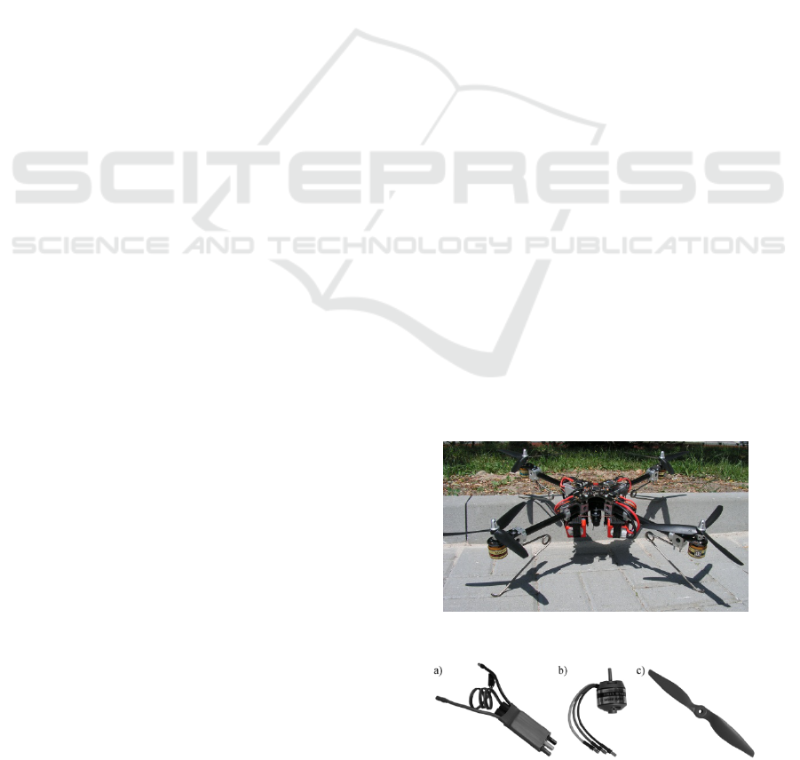
Figure 1: Hornet robot.
Figure 2: Speed controller (a), drive unit: brushless DC
engine (b) and propeller (c).
The CDM control according with the idea of robust
control does not enforce to obtain complica-ted and
complex mathematical model of the DU, but only
the simplest possible description, which accura-tely
245
Gardecki S., Giernacki W. and Goslinski J..
Speed Control of Drive Unit in Four-rotor Flying Robot.
DOI: 10.5220/0004477002450250
In Proceedings of the 10th International Conference on Informatics in Control, Automation and Robotics (ICINCO-2013), pages 245-250
ISBN: 978-989-8565-71-6
Copyright
c
2013 SCITEPRESS (Science and Technology Publications, Lda.)
reflects the dynamics. The aim of control algorithm
is then (in addition to stability and good quality of
control providing) a correction of impact of
nonmodeled and missed part of plant's dynamics –
therefore it was decided to use the experimental
method for determining DU’s model parameters
from its step response to the transfer function form.
2 ENGINE TEST STAND
For tests of high speed drive units, a special test
stand (TS) was built (Fig. 3), which enabled remote
control and measurements. In order to provide
constant and stable power supply to the DU, the
inRadio IN-450 power supply with high current
efficiency may be used, but during tests controller
drew power from 6000 mAh 11,1 V battery. The TS
was equipped with a set of sensors which allow to
control the power supply voltage of controller and to
measure of the DU current consumption, generated
thrust by the set of engine/propeller and the
rotational speed. The data from measurement system
were transmitted as a report to the computer applica-
tion, which was used as an setpoint adjuster and
controller (to set the same experimental conditions
for various power units). The signal sampling
frequency was equal to 300 Hz.
On the basis of earlier tests (Gardecki and
Kasiński, 2012) it was observed that despite the use
of the same BLDC engines and propellers, recorded
characteristics of drive units differ from each other,
which leads to stabilization difficulties of the robot
during the flight and reduces the flight time by
unfairly increase consumption of electricity. On this
reason authors opted for the synthesis of control
systems (with PID and CDM type controllers) for
particular DU. This paper considered results of
tuning for an exemplary, one of four drive units.
Two tests to provide a maximum knowledge
about modeled object were conducted. In the first
study, by the change of set voltage (fulfilment of
PWM) fed to the engine (in range from 0 to 100%,
step equal to 1%), characteristics of signals shown in
Fig. 4, were recorded. For the mass of the quadrotor
equal to 1,6 kg, the necessary and total thrust which
allows to overcome its force of gravity amounts
15,696 N. It should be noted that the maximum
thrust (19,09 N) of the tested DU is achieved at
PWM=77 %, RPM=8893 r/min and the current is
equal to I=15,551 A, but the maximum speed
RPM=9039 r/min is achieved at PWM=75 %, and
I=14,419 A. These parameters illustrate limits of
useful ranges during the operation of robot.
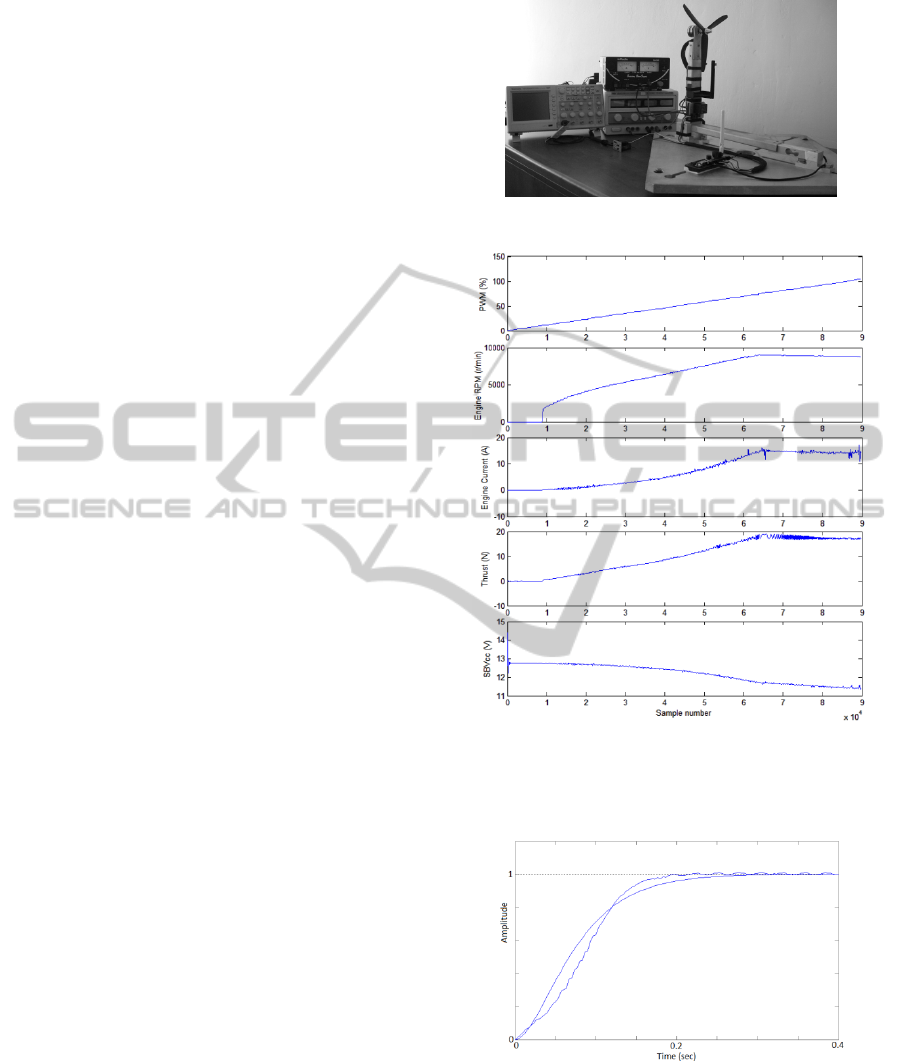
Figure 3: Engine test stand.
Figure 4: PWM (a), propeller rotational speed – RPM (b),
engine current (c), thrust of engine/propeller unit (d),
power supply voltage (e) in the function of control voltage
change from 0 to 5 V.
Figure 5: Model (smooth line) and robot step responses
matching.
In the second test a step response of modeled DU
has been observed (voltage changed from 0% to
100% PWM) to obtain the simplest plant model,
which is desirable for control system synthesis, but it
has to accurately reflect the particular DU dynamic,
ICINCO2013-10thInternationalConferenceonInformaticsinControl,AutomationandRobotics
246
which useful thrust starts from minimum value
3,924 N (RPM=4492,5 r/min). The time course of
rotational speed from Fig. 5 has been recorded and it
was decided to apply the second-order inertial plant
model (1), which parameters were determined by
step responses matching in experimental way.
22
11
()
0,0016 0,08 1
0,04 1
Gs
s
s
s
(1)
3 SYNTHESIS OF CDM AND PID
CONTROLLERS
CDM Control
The CDM algorithm is based on an idea of the use of
relationship between obtained closed-loop system
time characteristics and the placement of its
characteristic polynomial poles on the complex
plane s (Manabe, 1998). The control system under
consideration is presented in Fig. 6, where F(s) -
input numerator polynomial of controller transfer
function, A(s)/B(s) - numerator/denominator polyno-
mial of controller transfer function, N(s)/D(s) -
numerator/denominator of plant transfer function,
r(t)/y(t) - reference/output signal, e(t) - control error,
z(t) - external disturbance signal, v(t)/u(t) - un/con-
strained control signal, m(t) - measured noise signal.
A characteristic polynomial of closed-loop system
P(s) (of n-th degree) is defined by the equation (2):
0
() () () () () ,
n
i
i
i
Ps DsAs NsBs as
(2)
The synthesis of controller for system from Fig. 6
(with the use of CDM algorithm from Fig. 7) and
CDM procedure (Hamamci and Koksal, 2004) are
presented below.
A. Controller Synthesis
Notation of Plant Model with use of transfer
Function:
1
110
1
110
...
()
,
() ...
ll
ll
mm
mm
ns n s ns n
Ns
Ds d s d s ds d
(3)
where: l – degree of N(s) polynomial (less or equal
to m – degree of D(s) polynomial).
Choice of Controller Structure
Based on analysis of expected disturbances,
degrees of polynomials A(s) and B(s) are chosen
according to Table 1. Controller polynomials,
respectively degree: p and q are written in forms (4):
00
() , () .
pq
ii
ii
ii
A
slsBsks
(4)
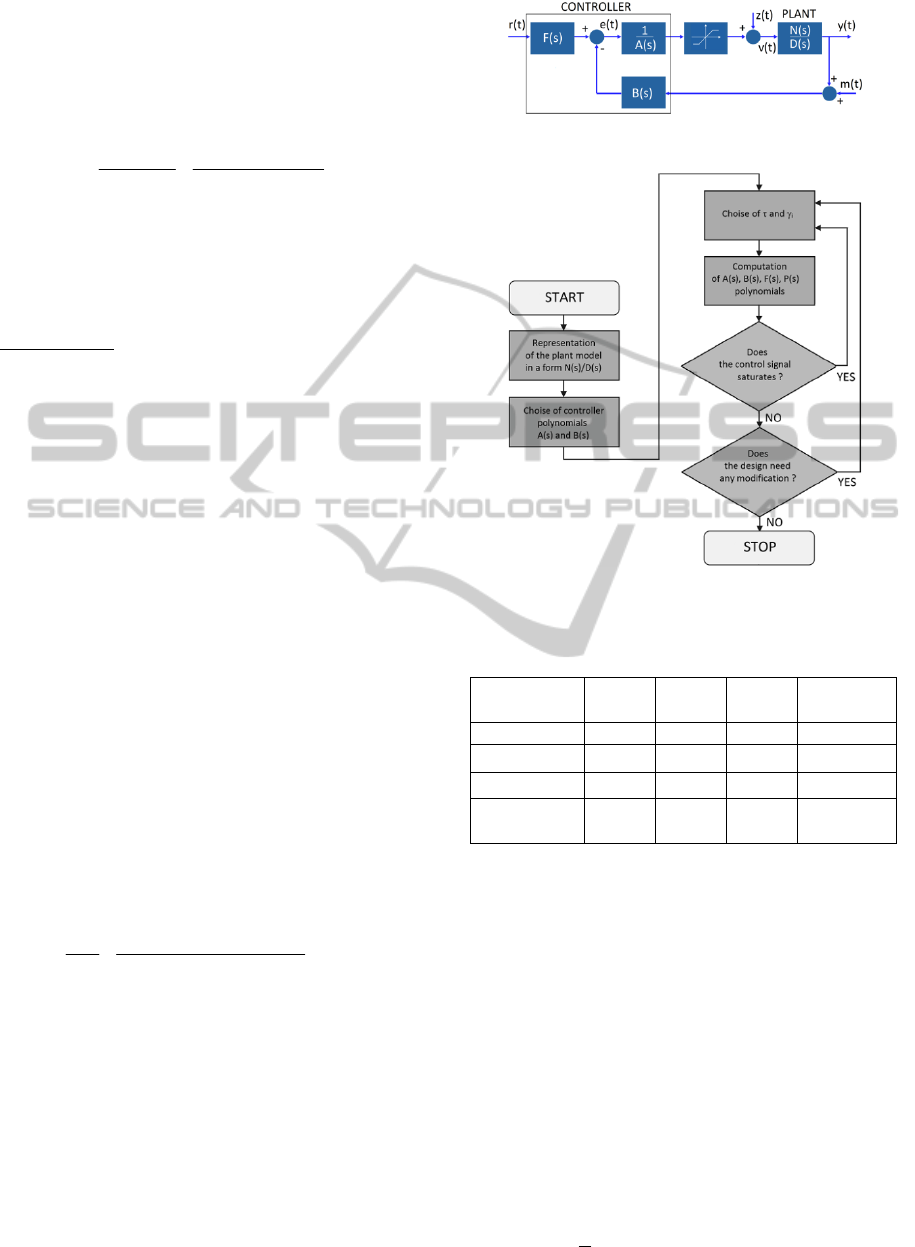
Figure 6: Block diagram of CDM control closed loop.
Figure 7: CDM algorithm.
Table 1: The choice of transfer function polynomials
degrees due to expected type of disturbances.
Type of
disturbance
Degree
of A(s)
Degree
of B(s)
Degree
of P(s)
Condition
None m-1 m-1 2m-1 -
Step m m 2m l
0
=0
Ramp m+1 m+1 2m+1 l
0
= l
1
=0
Impulse/
sinusoidal
m-1 m-1 2m-1 -
Choice of
and
i
Values
The CDM uses relationship (5) between the
equivalent of time constant (
) – used to build the
characteristic polynomial (P
T
) and the expected time
of step response (t
s
):
/2,5~3.
s
t
(5)
The advantage of proposed algorithm is Manabe
standard form (6) (vector specifying stability indices
-
i
). It represents system stability on a Coefficient
Diagram (CD) and defines the P
T
(s), which should
be used to ensure requirements of system dynamics
in the first iteration of algorithm. Standard forms
should be treated as initial setting values of each
index of stability - details in (Manabe, 1998).
2,5 2 2 ... 2
T
i
(6)
SpeedControlofDriveUnitinFour-rotorFlyingRobot
247
for i=1,…,n-1;
0
=
n
=
and n is P
T
(s) degree.
To specify numerically and graphically (on CD)
stability limit of system, equation (7) for stability
limits is used:
*
11
11
.
i
ii
(7)
Calculation of P(s), F(s), A(s) and B(s)
The equivalent of time constant and stability
indices building the target characteristic polynomial
(8), which is compared to equation (2), therefore
from diophantine equation (9) numerical values of
controller coefficients (l
i
and k
i
) may be calculated.
1
0
2
1
1
() 1
i
n
i
T
j
i
j
ij
Ps a s s
(8)
() ()
T
Ps P s
(9)
Polynomial F(s) is defined by the equation (10):
0
0
()
() .
()
s
s
Ps
Fs
Ns
(10)
Recurrence of CDM Algorithm
The option of procedure recurrence depends only
on the fact, whether a satisfactory control quality
was obtained (according to previously chosen
criterion e.g. size of the overshoot, saturation of
control signal, settling time of output signal,
specified limit of stability). By reduction of stability
limit or extension of the expected time of step
response, algorithm may be recurred. The CD
analysis is useful in this part of procedure.
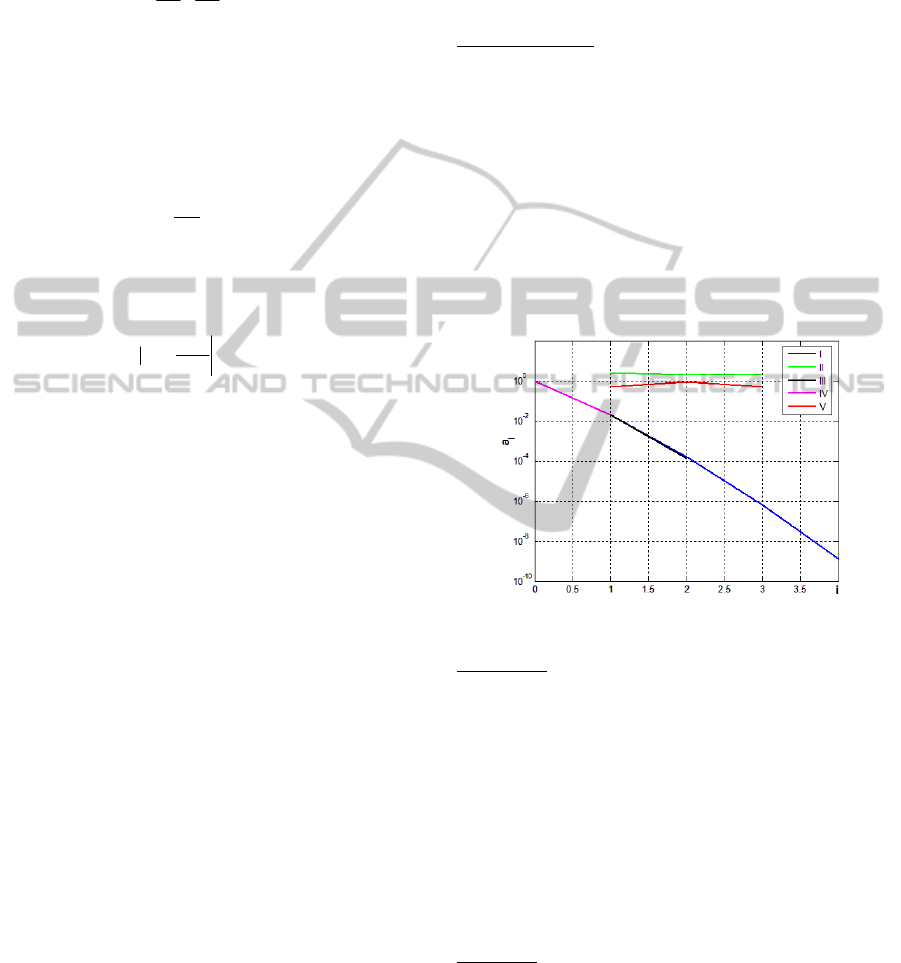
B. Coefficient Diagram
In synthesis and analysis of the control system based
on the CDM algorithm, half-logarithmic coefficient
diagram is used (Fig. 8), where the vertical axis
logarithmically shows coefficients of the
characteristic polynomial (a
i
), stability indices (
i
),
stability limits (
i
*) and the equivalent time constant
(
), while the horizontal axis shows the i values
corresponding to each coefficient.
In Fig. 8 number marks were introduced:
• numerical values (a
i
) of P
T
(s) coefficients – I,
• numerical values of stability indices (
i
) – II,
• numerical values (k
i
) of B(s) coefficients– III,
• equivalent of time constant (
) – IV,
• numerical values of stability limits (
i
*) – V.
By analogy with the Bode and Nyquist plots,
coefficient diagram provides the necessary
information about the system robustness, stability
and dynamics. The degree of convexity, which is
obtained from coefficients of the characteristic
polynomial, gives a measure of stability, while the
general inclination of the curve gives a measure of
the speed of response (Manabe, 1998). The variation
of the shape of the a
i
curve due to plant parameter
variation is a measure of robustness (Hamamci and
Koksal, 2004).
Stability analysis
For values
i
and
i
vertical distance between the II
and V curves is a measure of system stability (if the
distance for each i increases, then the system has
bigger stability limit). Analyzing the situation in the
complex plane s, this corresponds to the placement
of system poles in the left half-plane in larger
distance from the imaginary axis specifying the limit
of stability. It should be noted that the system is
stable only if curves do not cross each other and the
curve II is above the curve V (Manabe, 1998). The
basis of a theoretical analysis of a system stability is
Lipatov and Sokolov criterion.
Figure 8: Coefficient diagram of CDM system model (1).
Robustness
Assessment of system robustness is based on the
mutual position of I and III curves. If the curve III is
below the curve I, then the system is more robust to
parametric uncertainty – robustness increases when
the curves are closer to each other. It was shown in
(Manabe, 2010) that depending on the plant type, in
general, it is possible to design with the use of CDM
algorithm a control system, which is stable due to
the change the i-th characteristic polynomial
coefficient values in the range from 0,5 to 3 times in
relation to the nominal value of this factor.
Dynamics
Dynamics of system is characterized by the time
constant equivalent. The system is characterized by
higher dynamics for smaller values of
- in diagram
it corresponds to a larger angle of the curve IV
inclination. Analysis of the time constant equivalent
is also important in the case of control signal
constraints. If the control signal is saturated, then the
ICINCO2013-10thInternationalConferenceonInformaticsinControl,AutomationandRobotics
248
key issue in the control system synthesis is to return
to the stage of selection of expected equivalent time
constant value to increase this value (to slow down
the expected step response) and retry the algorithm.
The CDM controller was tune for possibility of
step type disturbance appearance (eg., blow of the
strong wind on the DU propellers). After the selec-
tion of appropriate controller structure (according to
the Table 1) for the model transfer function, the
Manabe standard form (6) was assumed. Then for
the chosen (expected) step response time t
s
=0,05
~0,06 sec, equivalent of time constant =0,02 sec
was calculated. The CDM controller was obtained:
2
2
( ) 0,0008 0,36 ,
( ) 0,0001 0,0196 1,
1.
A
sss
Bs s s
Fs
(11)
PID Control
To compare the control and tracking quality, the
second controller (PID - proportional-integral-
derivative), was used. Its parameters, namely the
gain of proportional part (k
P
), integral part (k
I
) and
derivative part (k
D
), were set in Simulink Response
Optimization tool – for similar assumptions as for
the CDM control. The optimization algorithm found
solution after 97 iterations (different controller sets)
as: k
P
=3,24, k
I
=49,40, k
D
=0,06. This controller
provides a step response after the time ~ 0,06 sec
with minimal overshoot (Fig. 9).
Figure 9: Step responses for CDM and PID controllers.
4 COMPARATIVE TESTS
Presented above control systems have been
implemented in the MATLAB 7.0/ Simulink under
OS Windows 7 system in default configuration.
Obtained results from numerical tests are presented
below. Parameters of PID and CDM control systems
remained constant in all performed tests. To control
quality assessment of the DU speed, except time
characteristics, integral quality indices were used:
IAE (integral of absolute value of error) and ISE
(integral of error squared).
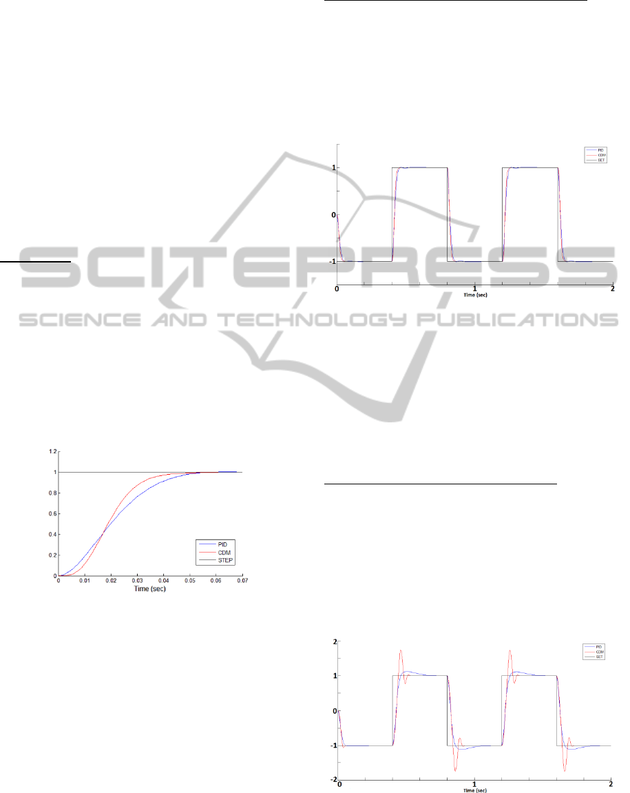
Tracking of Setpoint Signal in Nominal Systems
In the first stage of numerical tests, in systems
without disturbances and constraint of control signal
amplitude, tracking quality of set rectangular signal
(amplitude equal to 1, period to 0,8 sec, control
horizon to 2 sec), was tested. Signals are presented
in Fig. 10 and values of integral quality indices are:
- 1,925 (IAE) & 1,896 (ISE) for CDM,
- 1,903 (IAE) & 1,869 (ISE) for PID system.
Figure 10: Tracking of SET (setpoint) signal in PID and
CDM nominal systems.
The analysis of signals (Fig. 10) informs that despite
the use of optimization procedure to obtain the PID
controller and fulfilment of assumptions imposed on
the step response (Fig. 9), as well as marginally
lower values of IAE and ISE indices – PID
controller has an undesirable tendency to over-shoot,
which is not present in CDM control.
Tracking of Setpoint Signal at Constraints
In the second simulation test one imposed in both
control systems the same saturation of control signal
amplitude (u
max
=±6). All simulation parameters and
controllers remain unchanged in the relation to the
first test. The results are presented in the form of
reference and output signals (Fig. 11). Integral
quality indices were recorded and are equal
respectively to 1,968 (IAE) & 2,043 (ISE) for CDM
and 1,942 (IAE) & 1,963 (ISE) for PID controller.
Figure 11: Tracking of SET (setpoint) signal in PID and
CDM nominal systems at constraints - u
max
=±6.
SpeedControlofDriveUnitinFour-rotorFlyingRobot
249
Despite the fact that IAE and ISE values are
similar for both controllers, the analysis of Fig. 11
shows the differences in time curves of both output
signals – in the case of ideal (nominal) control
system with constraint of control signal amplitude –
PID controller produces significantly less overshoot,
but it needs almost twice as much time to bring
output signal value to the level of reference signal.
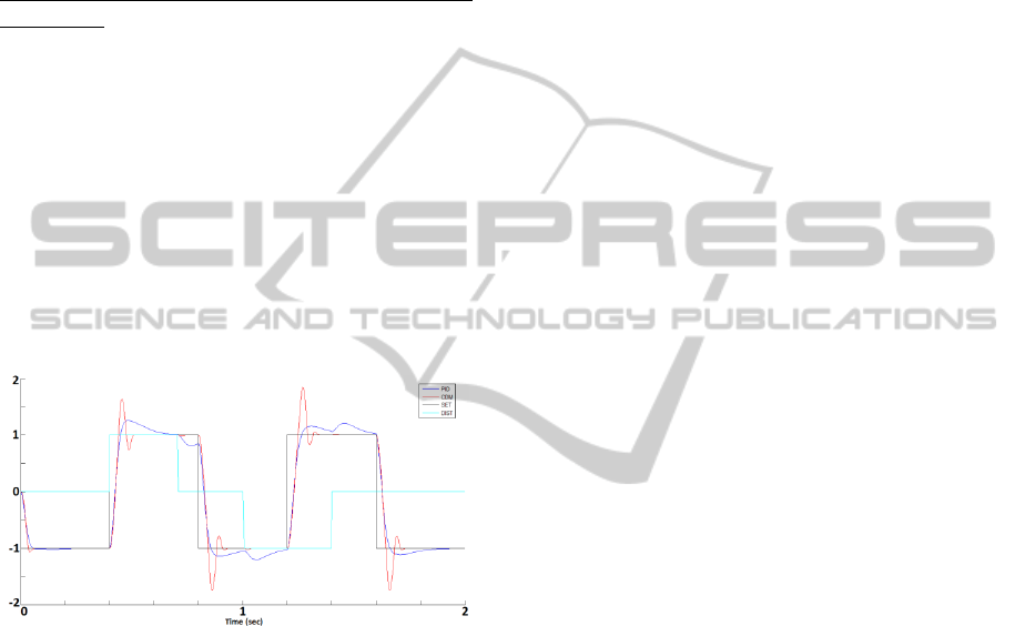
Tracking of Setpoint Signal in disturbed Systems at
Constraints
In the last test, an additional external disturbance
with step change of amplitude level over the time,
has been introduced to CDM and PID systems. The
quality of tracking was verified in the simulation
with similar parameters as in previous test. Values of
integral quality indices are equal respectively to
1,969 (IAE), 2,046 (ISE) for CDM controller and
1,995 (IAE), 2,082 (ISE) for PID. Results of
simulations (with external disturbance signal –
DIST) are presented in Fig. 12. In both cases, the
systems follow a setpoint signal, but for the CDM
control, the quality is definitely better – appearing
disturbances are damped much more quickly.
Figure 12: Tracking of SET (setpoint) signal in PID and
CDM disturbed systems at constraints - u
max
=±6.
5 CONCLUSIONS
Evaluation of the both presented control techniques
efficiency for variable speed control of the flying
robot DU is not easy and unambiguous, because of
robot’s control specificity as a complex dynamic
object. Its speed control is directly associated with
position and orientation, provided by the external
cascade controller which supports all four engines.
In planning of the minimum cost of energy
(minimizing the control signal changes frequency),
which is important from the perspective of the
limited length of flight (approx. 15 minutes) by the
battery power supply used in robot, it is reasonable
to select the PID controller, because it generates a
smooth transfer characteristics. The tendency to
overshoot can be eliminated by different method of
tuning than suggested in this article, such as swarm
optimization algorithm or genetic algorithms.
On the other hand so dynamic object as
quadrotor is very sensitive to transient environment-
tal conditions, such as wind and roll and it requires
very fast reactions. The CDM controller, which is
designed for the presence of step type disturbances,
during the third conducted test ensured generally
faster damping of disturbance effects as well as
better tracking quality through dynamic changes of
control signal. The overshoot that appears, should be
eliminated by the use of modified algorithm of the
CDM method. Such works had been already
conducted with the positive effects for other types of
objects – by using an additional block of pre-filter in
the controller, which parameters may be optimized
by the pole-colouring method (Bir et al., 2005).
The use of above proposed techniques of the PID
and CDM controller sets improvement is now a
starting point for further researches and
implementation tests on the real robot.
REFERENCES
Augugliaro, F., D’Andrea, R., Lupashin, S. and A.
Schöllig, 2010. Synchronizing the Motion of a
Quadrocopter to Music. In Proc. of the IEEE Inter.
Conf. on Robotics and Aut., Alaska, pp. 3355 – 3360.
Bir, A., Öcal, Ö. and M. T. Söylemez, 2005. Robust Pole
Assignment using Coefficient Diagram Method. In
Proc. of ACSE’05 Conf., Cairo, Egypt, CD.
Budiyono, A., 2005. Onboard Multivariable Controller
Design for a Small Scale Helicopter Using Coefficient
Diagram Method. In Proc. of the ICEST, Seoul, CD.
Gardecki, St. and A. Kasiński, 2012. Testing and selection
of electrical actuators for multi-rotor flying robot,
Measurements, Automation & Control, vol. 1, no. 1,
pp. 80-83.
Gertler, J., 2012. U. S. Unmanned Aerial Systems,
Congressional Research Service Report, USA.
Hamamci, S. E. and M. Koksal, 2004. A Program for the
Design of Linear Time Invariant Control Systems:
CDMCAD. Computer Applications in Engineering
Education, vol.12, no.3, pp. 165-174.
Manabe, S., 1998. Coefficient Diagram Method. In Proc.
of IFAC Automatic Control in Aerospace, Seoul, pp.
199-210.
Manabe, S., 2010. Coefficient Diagram Method for
Control system design, unpublished part of the
monograph provided by author.
Salih, A. L., Moghavvemi, M., Mohamed, H. A. F. and K.
S. Gaeid, 2010. Flight PID controller design for a
UAV quadrotor. Scientific Research and Essays, vol.
5, no. 23, pp. 3660-3667.
ICINCO2013-10thInternationalConferenceonInformaticsinControl,AutomationandRobotics
250
