
Robotic Pre-manipulation
Real-Time Polynomial Trajectory Control for Dynamic Object Interception with
Minimum Jerk
Arjun Nagendran
1
, Remo Pillat
1
and Robert Richardson
2
1
Institute for Simulation and Training, University of Central Florida, 3100 Technology Pkwy, Orlando, FL 32826, U.S.A.
2
School of Mechanical Engineering, University of Leeds, Leeds, LS2 9JT, U.K.
Keywords:
Object Capture, Trajectory Planning, Minimum-Jerk.
Abstract:
This paper presents a method for capturing a free-moving object in the presence of noise and uncertainty
with respect to its estimated position and velocity. The approach is based on Hermite polynomials and in-
volves matching the state-space parameters of the object and the end effector at the moment of contact. The
method involves real-time re-planning of the robot trajectory whenever new estimates of the object’s motion
parameters are available. Continuity in position, velocity, and acceleration is preserved independently of the
planning update rate and the resulting trajectories are characterized by low jerk. Compared to other methods
that directly solve for higher-order polynomial coefficients, the proposed algorithm is computationally effi-
cient and does not require a linear solver. Experimental results confirm the advantages of this method during
real-time interception of a dynamically moving object with continuous velocity estimation and high-frequency
re-planning.
1 INTRODUCTION
Robotic manipulation is an important problem in sev-
eral application domains. A prerequisite for robotic
manipulation is the ability to ’pick up’ an object. For
objects that are static in nature, this essentially re-
duces to a path planning problem for the end effector
of the robotic manipulator. Unless the environment
continuously changes, it is relatively straightforward
to pre-plan a path for the end effector while ensur-
ing smooth motions for the robotic arm. Moving ob-
jects present a special challenge, because they may
have to be intercepted or grasped before they can be
manipulated. Measurement uncertainties during path
planning of the robotic manipulator can result in rapid
changes in the motion profile of the system, thereby
subjecting the mechanism to jerk (third derivative of
position) and increasing wear on the system. Addi-
tionally, any mismatch in the velocities of the object
and the manipulator at the time of impact could cause
damage to the manipulator, captured object or both
entities.
“Minimum jerk trajectories are desirable for
their similarity to human movements and help im-
prove robot life-span by limiting robot vibrations ”
(Piazzi and Visioli, 1997)
Traditionally, higher-order polynomials are used
to minimize jerk during robotic motion, but are
mostly pre-planned with a priori knowledge of the tar-
get coordinates. When used in the time domain, the
coefficients of these curves can be varied to create a
motion profile for the end effector of a manipulator.
By choosing a polynomial with a sufficiently high de-
gree, it is possible to preserve continuity of its second
derivative, i.e. acceleration, thereby minimizing jerk.
Evaluating these higher-degree polynomials can how-
ever be computationally expensive. This is of particu-
lar interest since the coefficients of these polynomials
must be tuned so that the end effector motion profile
adapts to the (varying) velocity of an incoming object
in real-time and at potentially high update rates.
The contribution of this work is in achieving low-
jerk motion profiles for robotic end effectors while
ensuring minimum impact forces during interception
and capture. This is achieved by continuously match-
ing state-space parameters (position, velocity and ac-
celeration) between the object and the end effector at
the predicted rendezvous point. In contrast to existing
methods, the presented method has a high tolerance
for uncertainties and noise in the state space estimates
of the approaching object while being computational
efficient. The coefficients of a higher-order polynomi-
417
Nagendran A., Pillat R. and Richardson R..
Robotic Pre-manipulation - Real-Time Polynomial Trajectory Control for Dynamic Object Interception with Minimum Jerk.
DOI: 10.5220/0004478904170426
In Proceedings of the 10th International Conference on Informatics in Control, Automation and Robotics (ICINCO-2013), pages 417-426
ISBN: 978-989-8565-70-9
Copyright
c
2013 SCITEPRESS (Science and Technology Publications, Lda.)

als can be tuned in real-time and at high update rates
to ensure the successful interception of dynamic ob-
jects. A video demonstration of this capture process
can be viewed at http://youtu.be/yTx4a9UAMAM.
This paper describes the following:
• Choosing suitable polynomial trajectories that are
characterized by low-jerk and allow sufficient
flexibility to alter position, velocity and acceler-
ation while preserving continuity at every instant
in time during real-time capture.
• Re-computingthe polynomialtrajectories at every
instant in response to incoming velocity estimates
at a sampling frequency of 200 Hz.
• Reducing jerk during the entire process of inter-
ception, with the additional capability of extend-
ing the same acceleration profile for post-capture
(deceleration).
• Experimental testing and results of the method
during real-time interception of a dynamically
moving object with continuous velocity estima-
tion in the presence of noise.
2 BACKGROUND
During robotic interception and capture, a differ-
ence in velocity at the grasping instant may result
in slippage or impact which can cause damage
to the object or even damage to the manipulator
(Lin et al., 1989). Traditional methods of solving this
velocity matching problem involve predicting the po-
sition of an incoming object and positioning the end
effector at the computed interception point to capture
the object (Borg et al., 2002; Bauml et al., 2010).
Several path-planning techniques exist to achieve this
interception point including the use of polynomi-
als in general as described in (Croft et al., 1998;
Papadopoulos et al., 2005) and cubic splines
in specific (Gasparetto and Zanotto, 2008;
Wang and Horng, 1990). Many of these techniques
use a one-shot design approach for the polynomi-
als, assuming a priori knowledge of the incoming
object such as constant acceleration and velocity
(Campos et al., 2006) and resulting in pre-planned
trajectories for robotic interception. While these
methods are suitable in constrained environments
with repetitive tasks, the velocity of the incoming ob-
ject may change in unconstrained environments. The
capture of such objects presents a challenge due to a
continuously changing predicted interception point.
Additionally, with purely predictive interception
systems, impact and bounce are issues that must be
addressed. High speed robotics (Namiki et al., 2003;
Imai et al., 2004) overcomes the need for prediction
by simply reacting to the changing position estimates
of an object at a very high frequency. However,
no consideration of smoothness or jerk reduction is
possible with such systems.
Several researchers have previously addressed
the need for velocity matching. Nelson et.al.
(Nelson et al., 1995) emphasize in their work the need
for fast and stable transitions from non-contact states
to contact states, with minimum impact and bounce.
An approach where force and vision feedback are
simultaneously used to minimize the impact forces
when a stiff manipulator makes contact with a stiff
surface is presented. In effect, the static surface can
be thought of as having zero velocity and the manip-
ulator is forced to achieve minimum velocity just be-
fore contact. In (Lin et al., 1989), a coarse tuning al-
gorithm which drives the end effector into the neigh-
borhood of the object in minimum time, and a fine
tuning algorithm which ensures zero relative velocity
and acceleration at the time of grasping is presented.
A sensor based system employing the above method
is simulated for a two-degree of freedom (2DOF) pla-
nar robot at a sampling rate of 20 Hz.
The authors of (K¨ovecses et al., 1999) describe
the equations of the robotic end effector and object
independently before the interception phase. Ac-
cording to the authors, the dynamics are dependent
on the velocities and angular velocities at the in-
stant of contact. It is proved that when these com-
ponents are zero, there are no impulsive forces act-
ing on the system, resulting in a smooth capture.
(Zhang and Buehler, 1994) define a smooth grasp as
one in which the position, velocity and acceleration
of the robot end effector matches that of the moving
object at the point of contact.
While trying to achieve a certain end effector ve-
locity, it is important to be able to control its trajec-
tory. A trajectory defines the position, velocity and
accelerations of the end effector in its task space coor-
dinates. Confining the trajectory of the end effector to
be in line with the path of the object can significantly
help minimize the mismatch in velocities between the
two. Commonly used trajectories such as a linear tra-
jectory, with parabolic blends are subject to high jerk,
due to sudden changes in acceleration. The also re-
quire the application of an instantaneous change in
force by the actuator which is not practical. Other
methods of trajectory generation include third- and
fifth-order polynomials that describe the end effector
path in joint space; fifth-order polynomials have the
added advantage that they ensure low jerk values.
A third-order spline interpolation based trajectory
planning method to minimize the instantaneous ve-
locity change during bipedal robot foot contact is pro-
ICINCO2013-10thInternationalConferenceonInformaticsinControl,AutomationandRobotics
418
posed in (Tang et al., 2003). Simulation results reveal
that the trajectory obtained helps reduce impact. A
method for generating smooth jerk-bounded trajec-
tories is developed in (Macfarlane and Croft, 2003).
Jerk limitation results in improved tracking and re-
duced wear on the robot. The method used involves
the concatenation of fifth-order polynomials to gener-
ate a smooth trajectory between two way points.
The above methods require accurate and quick
control of the end effector to effectively match the ve-
locity of a moving object. The performanceis also de-
pendent on the actuator limits with respect to its abil-
ity to apply quick-changing forces. In keeping with
these, it is required to efficiently design polynomial
trajectories that are adaptive to changes in parametric
conditions of objects being captured in real-time. Ad-
ditionally, they must cope with changing parametric
estimates obtained from sensor data that are subject
to noise and uncertainties. This problem forms the
focus of this work.
3 FORMAL PROBLEM
DEFINITION
During robotic manipulation, a difference in veloc-
ities at the instant of grasping can result in impact,
which can cause the object being captured to bounce
off the end effector, and also cause damage to the ob-
ject or end effector. The effect of the difference in ve-
locities must therefore be understood, and a method to
minimize this mismatch must be developed to ensure
a successful grasp at the time of contact.
3.1 Velocity Matching and Impact:
Influence on Kinetic Energy
The velocity matching problem along a single axis is
illustrated in Figure 1. A mass M (kg) approaches
the end effector of a serial-link robotic arm with a
velocity V
mass
(m/s). The end effector cannot move
beyond its inner workspace limit D
lim
(m). The
mass is therefore required to be decelerated over a
distance D
stop
(m), a method for which was first
described in (Nagendran et al., 2007) and improved
upon in (Nagendran et al., 2011). From the known
velocity of the incoming mass, an intercept point for
the end effector and the object is computed (object
travels a distance D
intercept
(m) before impact). The
distance from the initial position of the end effector
(its outer workspace limit D (m) as measured from the
base coordinate frame) to the intercept point is given
as D
ef f
(m). The process of velocity matching re-
Figure 1: Illustration of the velocity matching problem
along a single axis.
quires some acceleration of the manipulator so that
the velocity of the end effector V
ef f
(m/s) matches
V
mass
(m/s) over this distance D
ef f
(m). Note that
the differences in effective distances covered by the
mass and the end effector from the start of the veloc-
ity matching process result in varied times over which
the same velocities need to be achieved.
When impact occurs, a portion of the kinetic en-
ergy of the two bodies is lost as thermal energy. Ac-
cording to Newtons experimental law (of impact /
restitution), the loss of kinetic energy after impact of
two straight point masses m
1
and m
2
with initial ve-
locities v
1
and v
2
can be determined using
L
ke
=
1
2
m
1
.m
2
m
1
+ m
2
(v
1
− v
2
)
2
(1− k
i
2
) (1)
where k
i
is the coefficient of impact and is depen-
dent on the material properties of m
1
and m
2
. It is
evident from Equation (1) that by minimizing the mis-
match in the velocities of the two objects, the impact
and hence the amount of kinetic energy lost can be
minimized. The impact therefore serves as a quantita-
tive measure of the performance of the velocity match
in the experimental trials discussed in Section 6.
3.2 Constraints for Successful Velocity
Matching
Let T be the time instant at which contact between
the end effector and the object occurs and t be the
continuous time axis.
• To ensure low impact during capture (and pre-
vent bounce), the position, velocity and accelera-
tion of the end effector must match that of the ob-
ject at the time of capture, i.e. e
obj
(T) = ˙e
obj
(T)
= ¨e
obj
(T) (Zhang and Buehler, 1994), where e
obj
represents the error between object and end effec-
tor state variables.
• Additionally, there must be no collision between
the object and the end effector prior to the time
taken by the object to reach the capture point.
RoboticPre-manipulation-Real-TimePolynomialTrajectoryControlforDynamicObjectInterceptionwithMinimumJerk
419

• Due to inherent actuator dynamics, there will be
errors between the desired and actual positions of
the end effector (e
ef f
). Ideally, these must be min-
imized during the process i.e. ∀t ≤ T, e
ef f
6= 0.
• The objective is to generate a position demand
for the end effector so as to minimize e
obj
(T),
˙e
obj
(T) and ¨e
obj
(T) within actuator limits. This
determines the time required to match the ob-
ject’s position, velocity and acceleration and also
the coordinate of the interception point in the
workspace of the manipulator.
4 POLYNOMIAL TRAJECTORIES
Previously published methods in the area of robotic
capture / interception generally assume a predictable
incoming object velocity (constant motion, decelera-
tion etc.) that serves as a basis for computing an in-
terception point during the maneuver. However, real-
world objects may not adhere to this assumption. Air
resistance, surface friction, and energy losses in kine-
matic components can all contribute to a variable ve-
locity. If the approaching object has a propulsion sys-
tem, any prediction of its future velocity is subject to
inaccuracy. Thus, adjustments to the end effector tra-
jectory need to be made continuously for successful
interception of the incoming object.
Ideally, the trajectory of the end effector can be
represented through a piecewise5th-order polynomial
to ensure a minimum jerk trajectory. The constraints
in order to perform velocity matching using this tra-
jectory include specifying the position, velocity and
acceleration at the initial and final positions of the
end effector. This can be done using quadratic or
cubic functions. However, since we require the ac-
celeration profile to be a third-order polynomial in
keeping with a minimum jerk trajectory, the desired
trajectory is represented as a 5th-order polynomial.
Solving for their coefficients in real-time is compu-
tationally expensive. By using the basis functions of
Hermite spline, the same solution can be found more
efficiently, thus allowing high-frequency re-planning
of the end effector motion profile. Please see Sec-
tion 4.2 for a comparison of computational efficiency
between the two methods.
4.1 Hermite Splines
Hermite polynomials are a specific set of orthogonal
basis functions whose linear combination spans the
space of all polynomials of a certain degree. The
splines are a piecewise concatenation of these poly-
nomials, each of which is in the Hermite form. De-
0 0.2 0.4 0.6 0.8 1
−0.5
0
0.5
1
1.5
2
Normalized Time
Position
Hermite Basis Functions
Interpolated Position
Figure 2: General example of quintic Hermite polynomial
interpolation. The Interpolated Position is a linear combi-
nation of the Hermite Basis Functions.
pending on the degree of the polynomials, continuity
in the derivatives will be preserved at the connecting
knot points. For the purposes of this work, quintic
Hermite splines will be considered, so minimum jerk
trajectories can be enforced. A quintic Hermite poly-
nomial is uniquely defined by a start and ending point
and the first two derivatives of the function at these
points.
For the normalized domain t ∈ [0,1], the quintic
Hermite basis functions h(t) take the following form:
h
0
(t) = −6t
5
+ 15t
4
− 10t
3
+ 1
h
1
(t) = −3t
5
+ 8t
4
− 6t
3
+ t
h
2
(t) = −0.5t
5
+ 1.5t
4
− 1.5t
3
+ 0.5t
2
h
3
(t) = 0.5t
5
− t
4
+ 0.5t
3
h
4
(t) = −3t
5
+ 7t
4
− 4t
3
h
5
(t) = 6t
5
− 15t
4
+ 10t
3
(2)
In the general case, the start and end time of a tra-
jectory segment are denoted as t
0
and t
f
. x
0
, v
0
and a
0
define the initial position, velocity, and acceleration at
t
0
, while x
f
, v
f
and a
f
denote their final values at t
f
.
For a given time t
h
∈ [t
0
,t
f
], the corresponding
normalized time in the [0,1] domain can be found
through:
t =
t
h
− t
0
∆t
(3)
Here ∆t = t
f
−t
0
is the conversion factor between
real and normalized time, but can also be used to
normalize and de-normalize velocity and acceleration
values. The actual position x and velocity v at this
normalized time t can then be calculated. For nota-
tional simplicity it is assumed that p, v, h, and
˙
h are
all functions of t.
x = x
0
h
0
+ v
0
h
1
+ a
0
h
2
+ a
f
h
3
+ v
f
h
4
+ x
f
h
5
v
n
= x
0
˙
h
0
+ v
0
˙
h
1
+ a
0
˙
h
2
+ a
f
˙
h
3
+ v
f
˙
h
4
+ x
f
˙
h
5
v = v
n
/∆t (4)
ICINCO2013-10thInternationalConferenceonInformaticsinControl,AutomationandRobotics
420

The derivatives
˙
h
0
...
˙
h
5
can be found analytically.
Similar expressions to Equation (4) can be derived for
the end effector acceleration and jerk.
4.2 Computational Efficiency of
Hermite Solution
Looking at Equation (4), it becomes immediately
clear that the calculation of a demand position and
demand velocity for any normalized time t involves
nothing more than a fixed number of multiplications
and additions. Furthermore, the computational com-
plexity is constant regardless of changing start and
end conditions. In the case of the pure fifth-order
polynomial solution, a new set of coefficients would
have to be calculated each time one of the variables
x
0
,x
f
,v
0
,v
f
,a
0
,a
f
changes.
To quantify the computational efficiency of the
Hermite-spline-based solution, a test program was
written in Matlab. Random vectors with 1 million ele-
ments were generated for the t
0
,t
f
,x
0
,x
f
,v
0
,v
f
,a
0
,a
f
parameters. There is an additional vector t with the
same number of elements that represents a random
time sample between t
0
and t
f
that is evaluated. Two
different methods for calculating the end effector tra-
jectory were implemented:
1. Linear Solver: The coefficients of the fifth-order
polynomial can be found by solving a system of
six linear equations. This method uses Matlab’s
optimized ’linsolve’ function that is based on LU-
decomposition. Using these coefficients, position,
velocity, acceleration, and jerk can be evaluated
for time instants t.
2. Hermite-based Solver: Based on Equation (4)
and the corresponding calculations for accelera-
tion and jerk, the end effector state for time in-
stants t can be directly identified.
Both solvers were executed on each of the 1 mil-
lion test cases and their respective runtimes recorded.
It should be noted that both solutions result in pre-
cisely the same trajectory solutions, but their runtime
differs. On a Core i7 processor with an operating
frequency of 3.2 GHz, the average time required per
iteration for solver (1) was 0.085 ms, whereas the
Hermite-based solver (2) executes in 0.017 ms on av-
erage. The Hermite splines thus provide a speedup of
almost 5 times over the linear solver.
It should be pointed out that the computational ad-
vantage is a requirement given the constantly chang-
ing start and end conditions due to noisy state esti-
mates of the approaching object. If a continuous es-
timation and adjustment of the trajectory is desired,
then the Hermite spline solution lends itself as an im-
plementation of choice. Each time a new estimate
of the approaching object’s position and velocity is
available, the current position, velocity, and acceler-
ation of the actuator can be used as initial conditions
for a new Hermite polynomial.
In addition, no linear solver is required for the
Hermite solution, so implementation can be simpli-
fied if executing on resource-constrained embedded
hardware.
4.3 Analysis: Hermite Splines for
Velocity Matching
The following section discusses the effect of continu-
ally changing velocities on the motion profile of an
end effector computed using Hermite splines. By
adaptively changing the motion profile of the end ef-
fector to incoming velocity estimates, a smooth mo-
tion profile for the end effector can be achieved. As
an added advantage, the velocity matching controller
does not require these updates at a fixed frequency; a
new estimate of the object’s velocity can be used as
soon as it is available thereby making the controller
robust to data loss and sensor noise.
0 0.2 0.4 0.6 0.8 1
0
0.05
0.1
0.15
0.2
0.25
0.3
0.35
Time (in s)
Position (in m)
Noiseless Hermite
Hermite Spline w/ 25% Noise on xf
0 0.2 0.4 0.6 0.8 1
−0.1
0
0.1
0.2
0.3
0.4
0.5
0.6
Time (in s)
Velocity (in m/s)
Noiseless Hermite
Hermite Spline w/ 25% Noise on xf
Figure 3: Achieving new motion profiles using Hermite
splines in the presence of noise.
The quintic Hermite basis functions are first com-
puted for a given instant in time as described by Equa-
tion (2). Equation (4) is then used to compute a de-
mand position and demand velocity for the end effec-
tor at every instant in time. Figure 4 illustrates the
process graphically. An initial estimate of the motion
profile for the end effector is used to compute the her-
mite spline that achieves 0.225m in 0.5s. At t = 0.2s,
a new estimate is acquired which requires the end ef-
fector to be positioned at 0.275m at t = 0.5s. The co-
efficients of the hermite spline are computed for the
new estimates resulting in a new ’blended’ hermite
spline as seen in the figure. Notice the continuity in
position and smooth changing velocity at t = 0.2s de-
spite the jump in target coordinate (by 22%). The
acceleration profile and jerk profiles also reflect these
changes but are still within acceptable limits and show
no large spikes. Figure 3 shows the position and ve-
locity profiles generated in the presence of 25% Gaus-
RoboticPre-manipulation-Real-TimePolynomialTrajectoryControlforDynamicObjectInterceptionwithMinimumJerk
421
0 0.05 0.1 0.15 0.2 0.25 0.3 0.35 0.4 0.45 0.5
0
0.05
0.1
0.15
0.2
0.25
0.3
0.35
Position of End Effector
Time (in s)
Position (in m)
0 0.05 0.1 0.15 0.2 0.25 0.3 0.35 0.4 0.45 0.5
0
0.2
0.4
0.6
0.8
1
Velocity of End Effector
Time (in s)
Velocity (in m/s)
0 0.05 0.1 0.15 0.2 0.25 0.3 0.35 0.4 0.45 0.5
−8
−6
−4
−2
0
2
4
6
Acceleration of End Effector
Time (in s)
Acceleration (in m/s
2
)
0 0.05 0.1 0.15 0.2 0.25 0.3 0.35 0.4 0.45 0.5
−100
−50
0
50
100
150
200
250
Jerk of End Effector
Time (in s)
Jerk (in m/s
3
)
Hermite Target − 0.275m
Newly Computed Hermite
Hermite Target − 0.225m
Hermite Target − 0.275m
Newly Computed Hermite
Hermite Target − 0.225m
Hermite Target − 0.275m
Newly Computed Hermite
Hermite Target − 0.225m
Hermite Target − 0.275m
Newly Computed Hermite
Hermite Target − 0.225m
New Estimate
New Target
Transition Point
Figure 4: Motion profiles of end effector during hermite blending.
sian, zero-mean, additive noise on the end position
estimate x
f
= 250 mm. A new Hermite spline is esti-
mated at each 0.05 s time step, starting from the cur-
rent position, velocity, and acceleration. The resulting
motion profile of the end effector is still smooth and
can therefore be altered in real-time without causing
large changes in acceleration or jerk during the pro-
cess. The velocity spikes at the end of the trajectory
are due to the relativelydrastic changes to x
f
that need
to occur in a shorter and shorter time span. To avoid
this behavior in real experiments, it is recommended
to cease the Hermite interpolation when the object is
within a small band before the target.
5 EXPERIMENTAL SETUP
An overview of the experimental setup showing the
hardware components (Table 1) is depicted in Fig-
ure 5. The mechanism used to illustrate the velocity
matching controller in the experiments is a 1 degree-
of-freedom (DOF) LinMot linear actuator. The Lin-
Mot is an electromagnetic device that can move a
slider linearly without the use of screws or gears. Its
position can be resolved with high accuracy within
0.05 mm. This is representative of the end effector
position along a single axis (see Figure 1) that can be
extended to serial link manipulators as desired. An
uniaxial force sensor from Transducer Techniques is
mounted at the end of the slider and used to record
forces encountered when in object contact. Desired
positions and velocities are commanded to the actua-
tor at a constant sampling frequency of 200 Hz. On
a lower level, this control mode circumvents any sec-
ondary motion planning, but the smoothness and fea-
sibility of the input trajectory has to be ensured by the
implemented motion controller.
Two separate carts were used as objects approach-
ing the actuator. One of the carts can be remotely-
driven at discrete constant velocities, while the other
is free moving. The free-moving cart is rolled down
a ramp towards the end effector and sometimes im-
peded using undulations as shown in Figure 5. One
wheel shaft on each robot is rigidly connected to
an incremental, quadrature optical encoder that pro-
duces 90 pulses per revolution. The encoder pulses
are counted by an Arduino microcontroller board and
wirelessly sent to the controlling computer via an
XBee RF module. This information is used to com-
pute the incoming velocity of the cart.
The velocity matching controller is implemented
in Labview and sends a position and velocity com-
mand stream to the Linmot actuator over a CAN
bus interface. The minimum-jerk trajectory is cal-
culated at 200 Hz and the actual position and veloc-
ity on the currently active 5th order polynomial is
sent to the Linmot actuator. The force sensor is read
through a National Instruments data acquisition board
at 200 Hz.
An ideal controller would execute the velocity
matching process as illustrated in Figure 6. When
the cart approaches the end effector, the linear actu-
ICINCO2013-10thInternationalConferenceonInformaticsinControl,AutomationandRobotics
422
Table 1: Hardware Components.
Image Component Description Function Specifications
(A) Linear Actuator (LinMot) PS01-23x160 sta-
tor with PL01-12x760/710 Slider
Implements end effector motion profile (us-
ing a closed-loop PID Controller)
Sampling Frequency: 200 Hz
Max. Velocity: 3 m/s
(B, C) Carts (VEX)
(a) Remote-controlled with discrete velocity
(b) Free-Moving (rolled down a ramp)
(a) Constant Velocity with single transition
(b) Continuously changing velocity
(D) Optical Shaft Quadrature Encoder (VEX) Measures velocity of incoming object / cart
(for real-time Polynomial Tuning)
Sampling Frequency: Velocity-dependent
Resolution: 90 ticks/revolution
(E) Uni-axial Force Sensor MDB-25 (Transducer
Techniques)
Measures impact of incoming object with end
effector (for theoretical verification)
Sampling Frequency: 200 Hz
Max. Force: 111.20N
(F) PointGrey Flea2 FL2-03S2C-C Captures final frames prior to impact (for data
review)
Frame Rate: 140 fps
Resolution: 640 x 160
(G) Custom Photo-Diode Beam Breaker Circuit Provides reference position and initial veloc-
ity estimate of incoming object
Sampling Frequency: 200 Hz
Output Voltage: 2.2V – 4.5V
Figure 5: The experimental setup with linear actuator, adjustable ramp, and mobile robots.
ator would execute a smooth trajectory to match the
cart’s position, velocity, and acceleration at the cap-
ture point. Once contact is established, the object can
be decelerated in a predefined workspace such as that
described in (Nagendran et al., 2011).
6 RESULTS
Several experimental trials were conducted to illus-
trate the repeatability and robustness of the controller
to continually changing velocity estimates prior to in-
terception. To illustrate the need for a continuously
updated motion trajectory, an experiment that relies
on a single measurement of the object’s velocity is
first described and analyzed. This is representative
of a single-shot capture approach where an incoming
object’s velocity is known beforehand and planning
occurs based on this apriori estimate. Experiments
that involved constant velocity motion (from the re-
motely operated cart) and changing velocity motion
(from the free moving cart, rolled down the ramp)
were conducted. Results presented below focus on
the free-moving scenario, since the constant velocity
case is fairly trivial to handle.
Figure 6: A typical velocity matching maneuver. The cart
approaches the end effector in the topmost image, while
the middle image shows the moment when contact is es-
tablished. The cart is decelerated and comes to rest in the
position shown in the bottom photo.
6.1 One-time Velocity Estimate
A single-shot approach is subject to failure in two in-
stances i.e. the incoming object’s velocity may either
be (a) lower or (b) higher than originally estimated.
In the former case, capture may never occur within
RoboticPre-manipulation-Real-TimePolynomialTrajectoryControlforDynamicObjectInterceptionwithMinimumJerk
423
the pre-defined distance while in the latter case, cap-
ture occurs prior to the pre-defined interception point,
resulting in a high impact force. The latter case is con-
sidered for analysis in this subsection. An ideal point
in the workspace of the LinMot is identified as the in-
terception (capture) point. This, for instance, can be
chosen depending on the portion of the workspace re-
quired for deceleration of the object. A beam-breaker
circuit (with photo-diode) is used to estimate the ve-
locity of the incoming cart and passed to the Hermite
polynomial trajectory planner. Based on this received
data, the time-to-impact is used to plan a minimum-
jerk spline to catch the object at the ‘target point’.
12.5 13 13.5 14 14.5
−0.5
0
0.5
1
1.5
Time (s)
Velocity (m/s)
End Effector
Cart
Contact Point
Target Point
Figure 7: Velocity graphs reveal a mismatch due to an early
contact between incoming object and end effector.
12.5 13 13.5 14 14.5
−2.0
0.0
2.0
4.0
6.0
8.0
10.0
Time (s)
End Effector Force (N)
Figure 8: Corresponding force graph reveals a large impact
force due to the mismatch in velocities.
Figure 7 shows the velocity graphs of the incom-
ing cart and the end effector during a failed inter-
ception scenario. The LinMot receives a one-time
estimate of the cart’s velocity, which is lower than
the subsequent velocity achieved by the cart. .The
planned motion is such that this velocity is achieved
overa pre-defined distance of 0.225 m in the LinMot’s
workspace, with the time-to-impact calculated based
on the distance of the cart. The cart’s higher veloc-
ity results in interception at a co-ordinate well before
the 0.225 m target is achieved, since the time to con-
tact is much lesser than originally estimated. The re-
sult is a high impact force, as seen in Figure 8 due
to the mismatch in velocities at the point of contact,
and consequently a higher jerk due to the change in
acceleration.
6.2 Continuous Velocity Estimate
In order to minimize impact and reduce jerk, it is re-
quired to continuously adapt the end effector’s mo-
tion to match the incoming object’s velocity. While
doing so, it is required to ensure smooth motion,
without discrete changes in acceleration that result in
jerk. This is implemented with the Hermite Spline
solution discussed in Section 4.3 at a frequency of
200 Hz. Several runs at different incoming veloci-
ties were conducted by varying the angle of the ramp
that was used to launch the cart towards the end effec-
tor. Five separate runs were executed for each experi-
mental condition and results are tabulated in Table 2.
The mean and standard deviation for different metrics
are shown and the important fields i.e velocity match-
ing percentage and the impact force are indicated by
shaded cells. In all conditions the velocities between
linear actuator and cart were matched to within 7.5 %
and the quality of the match is maintained through a
range of different absolute velocity magnitudes. The
force encountered on impact is on average less than
0.872 N, with conditions 1 and 3 showing even better
results. These experiments verify the quality of the
presented object capture method.
To further demonstrate how the presented method
copes with uncertainty in the velocity estimates, sev-
eral runs from Condition 3 will be analyzed. In the
experimental setup, two undulations of varying mag-
nitude (Figure 5) were placed in the path of the in-
coming cart, causing it to unevenly decelerate as it
approached the end effector. Velocity estimates in this
case could also degrade due to skipped encoder counts
when the undulations are traversed.
Several results from this run are shown in Figure 9
and analyzed in detail. To evaluate the quality of
the velocity matching at this target location, veloci-
ties of end effector and cart against time are plotted
in Figure 9a. At the impact time of 25.9 s, the linear
actuator’s velocity is 0.4135 m/s
2
, while the cart’s ve-
locity is 0.436 m/s
2
- a velocity mismatch of approx-
imately 5.2%. The positions of the cart and the linear
actuator are displayed in Figure 9(b). Performance is
further analysed by measuring the force encountered
on impact of the cart. Figure 9(c) shows the value of
the measured forces throughout the run. At time of
impact, the force is evaluated to 0.428 N. Compare
this with the significantly higher value described in
the failure case above. Please note that, for visual-
ization clarity, the force data has been filtered with a
low pass Butterworth filter. It should be pointed out
ICINCO2013-10thInternationalConferenceonInformaticsinControl,AutomationandRobotics
424

Table 2: Results of adaptive velocity matching experiments. Five runs were executed in each experimental condition.
Condition 1 Condition 2 Condition 3
mean stdev mean stdev mean stdev
Contact Point (m) 0.196 0.018 0.179 0.008 0.199 0.018
Contact Linmot Velocity (m/s) 0.221 0.026 0.380 0.028 0.345 0.038
Contact Cart Velocity (m/s) 0.239 0.023 0.401 0.025 0.353 0.045
Velocity Match (%) 92.540 2.212 94.591 1.374 96.328 2.266
Impact Force (N) 0.537 0.233 0.872 0.106 0.413 0.094
that these promising results are achieved in the pres-
ence of a constantly changing estimate for the time to
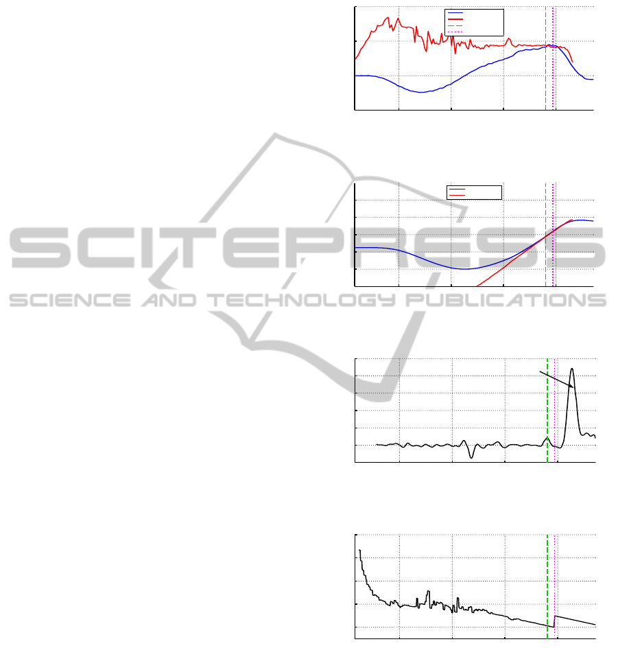
impact (see Figure 9(d)).
7 DISCUSSION, CONCLUSION
AND FUTURE WORK
In this work, a new approach to robotic interception
of moving objects was proposed. The method relies
on the use of higher order polynomials that exhibit
low jerk properties for continuous real-time trajec-
tory planning of robotic end effectors. In specific, the
use of Hermite splines for catching moving objects
in the presence of sensor noise was discussed. Re-
sults reveal a high accuracy of velocity matching prior
to interception resulting in low impact and reduced
jerk. Additionally, continuity of the end effector state-
space variables (up to the second derivative) are main-
tained during the process and can be extended to the
post-capture stage of robotic interception. Although
Hermite splines have attractive properties (see Sec-
tion 4.1), they have some drawbacks when used for
generating trajectories:
• The start and end constraints are guaranteed to be
fulfilled, but over and undershoot inside the inter-
polation interval can occur. This is problematic if
the actuator has fixed motion constraints.
• There is no way to constrain derivatives during in-
terpolation. For example, it is possible for com-
manded velocities to exceed the capabilities of the
actuator. Since the solution of the Hermite poly-
nomial is unique, there is no way to “adjust” or
re-calculate the trajectory with identical start and
end conditions. What we are looking for in this
case is a monotonic interpolation solution.
• The values on the spline are subject to oscillations
if the time between x
0
and x
f
is very small. For
instance, it may be noted that in Figure 3(b), oscil-
lations are amplified towards the very end, when
noise levels are high. This is particularly pro-
nounced due to the high order of the polynomial
(5th). Although this can potentially be rectified by
decreasing the order of the Hermite polynomial
selectively, the minimum jerk requirement cannot
be enforced in this case.
Several of the fore-mentioned issues are due to the
fact that Hermite polynomials are direct interpola-
tion functions, i.e. the interpolant function will di-
rectly pass through all knot or control points. B´ezier
Splines, that are ‘parametric’ curves provide a poten-
tial remedy to these problems by virtue of some of
their unique properties: The start and end conditions
can still be constrained by the position of two con-
trol points, but additional control points (that in gen-
eral do not lie on the interpolant) not only specify the
value of derivatives but also define an envelope, or
convex hull. It is guaranteed that between the start
and end point, the B´ezier curve is always contained
within that envelope. The calculation of the interme-
diate values is accomplished through De Casteljau’s
Algorithm, but is potentially more computationally
expensive compared to the Hermite splines. Design-
ing these B´ezier curves for this problem and inves-
tigating the fore-mentioned claim form a part of the
future and ongoing research directions of this work.
REFERENCES
Bauml, B., Wimbock, T., and Hirzinger, G. (2010). Kine-
matically Optimal Catching a Flying Ball with a
Hand-Arm-System. In International Conference on
Intelligent Robots and Systems (IROS), pages 2592–
2599. IEEE.
Borg, J., Mehrandezh, M., Fenton, R. G., and Benhabib,
B. (2002). Navigation-Guidance-Based Robotic In-
terception of Moving Objects in Industrial Settings.
Journal of Intelligent & Robotic Systems, 33(1):1–23.
Campos, J. A. F., Romo, S. R., Orozco, O. I., and Ortega,
J. L. V. (2006). Robot Trajectory Planning for Mul-
tiple 2D Moving Objects Interception: A Functional
Approach. In Electronics, Robotics and Automotive
Mechanics Conference (CERMA), volume 1, pages
77–82. IEEE.
Croft, E. A., Fenton, R. G., and Benhabib, B. (1998). Op-
timal Rendezvous-Point Selection for Robotic Inter-
ception of Moving Objects. IEEE Transactions on
Systems, Man, and Cybernetics. Part B, Cybernetics,
28(2):192–204.
Gasparetto, A. and Zanotto, V. (2008). A Technique
for Time-Jerk Optimal Planning of Robot Trajecto-
ries. Robotics and Computer-Integrated Manufactur-
ing, 24(3):415–426.
RoboticPre-manipulation-Real-TimePolynomialTrajectoryControlforDynamicObjectInterceptionwithMinimumJerk
425
Imai, Y., Namiki, A., Hashimoto, K., and Ishikawa, M.
(2004). Dynamic Active Catching using a High-Speed
Multifingered Hand and a High-Speed Vision System.
In International Conference on Robotics and Automa-
tion (ICRA), pages 1849–1854. IEEE.
K¨ovecses, J., Cleghorn, W. L., and Fenton, R. G. (1999).
Dynamic Modeling and Analysis of a Robot Ma-
nipulator Intercepting and Capturing a Moving Ob-
ject , with the Consideration of Structural Flexibility.
Multibody System Dynamics, 3(2):137–162.
Lin, Z., Zeman, V., and Patel, R. (1989). On-line Robot
Trajectory Planning for Catching a Moving Object. In
International Conference on Robotics and Automation
(ICRA), pages 1726–1731. IEEE Comput. Soc. Press.
Macfarlane, S. and Croft, E. A. (2003). Jerk-Bounded Ma-
nipulator Trajectory Planning: Design for Real-Time
Applications. IEEE Transactions on Robotics and
Automation, 19(1):42–52.
Nagendran, A., Crowther, W., and Richardson, R. C.
(2011). Dynamic Capture of Free-Moving Objects.
Proceedings of the Institution of Mechanical Engi-
neers, Part I: Journal of Systems and Control Engi-
neering, 225(8):1054–1067.
Nagendran, A., Richardson, R., and Crowther, W. (2007).
Bell Shaped Impedance Control to Minimize Jerk
While Capturing Delicate Moving Objects. In Pro-
ceedings of ICINCO-RA, pages 504–511.
Namiki, A., Imai, Y., Ishikawa, M., and Kaneko, M. (2003).
Development of a High-Speed Multifingered Hand
System and its Application to Catching. In Interna-
tional Conference on Intelligent Robots and Systems
(IROS), volume 3, pages 2666–2671. IEEE.
Nelson, B., Morrow, J., and Khosla, P. (1995). Fast Sta-
ble Contact Transitions with a Stiff Manipulator using
Force and Vision Feedback. In International Confer-
ence on Intelligent Robots and Systems (IROS), pages
90–95. IEEE Comput. Soc. Press.
Papadopoulos, E., Tortopidis, I., and Nanos, K. (2005).
Smooth Planning for Free-floating Space Robots Us-
ing Polynomials. In International Conference on
Robotics and Automation (ICRA), pages 4272–4277.
IEEE.
Piazzi, A. and Visioli, A. (1997). An Interval Algorithm
for Minimum-Jerk Trajectory Planning of Robot Ma-
nipulators. In Conference on Decision and Control
(CDC), volume 2, pages 1924–1927. IEEE.
Tang, Z., Zhou, C., and Sun, Z. (2003). Trajectory Plan-
ning for Smooth Transition of a Biped Robot. In In-
ternational Conference on Robotics and Automation
(ICRA), pages 2455–2460. IEEE.
Wang, C.-H. and Horng, J.-G. (1990). Constrained
minimum-time path planning for robot manipulators
via virtual knots of the cubic B-spline functions.
IEEE Transactions on Automatic Control, 35(5):573–
577.
Zhang, M. and Buehler, M. (1994). Sensor-based Online
Trajectory Generation for Smoothly Grasping Moving
Objects. In International Symposium on Intelligent
Control, pages 141–146. IEEE.
APPENDIX
24.5 25 25.5 26
−0.5
0
0.5
1
Time (s)
Velocity (m/s)
End Effector
Cart
Contact Point
Target Point
(a) The velocities of the cart and the end effector
throughout the run.
24.5 25 25.5 26
−0.1
0
0.1
0.2
0.3
0.4
Time (s)
Position (m)
End Effector
Cart
(b) The positions of the cart and the end effector through-
out the run.
24.5 25 25.5 26
−1.0
0.0
1.0
2.0
3.0
4.0
5.0
Time (s)
End Effector Force (N)
Force During
Deceleration
(c) The force encountered at the end effector during the
run.
24.5 25 25.5 26
−0.5
0
1
2
3
4
Time (s)
Time to Impact (s)
(d) The changing estimates for the remaining time to im-
pact.
Figure 9: Behavior of velocity matching controller when
estimated cart velocity changes unpredictably. Please note
that in all subfigures, the desired contact position (Tar-
get Point) and actual contact position (Contact Point) are
marked by vertical lines.
ICINCO2013-10thInternationalConferenceonInformaticsinControl,AutomationandRobotics
426
