A Bayesian Approach to Modeling Dynamical Systems in the Social

Sciences

Shyam Ranganathan

, Viktoria Spaiser

and David J. T. Sumpter

1,2

Department of Mathematics, Uppsala University, Uppsala, Sweden

Institute for Futures Studies, Stockholm, Sweden

Keywords:

Bayesian Methods, Model Selection, Dynamical Systems, Mathematical Modeling, Social Sciences.

Abstract:

The paper presents a new modeling approach using longitudinal or panel data to study social phenomena

and to make predictions of dynamic changes. While the most common way in social sciences to study the

relations between variables is using regression, our modeling approach describes the changes in variables as

a function of all included variables, using differential equations with polynomial terms that capture linear

and/or nonlinear effects. The mathematical models represented by these differential equations are derived

directly from data. The models can then be run forward to forecast future changes. A two-step model-ﬁtting

approach is applied to identify the best-ﬁt models and included visualisation methods based on phase portraits

help to illustrate modeling results. We show this approach on an example relating democracy to economic

growth.

1 INTRODUCTION

Since the 1960s when James S. Coleman published

his book an mathematical sociology (Coleman, 1964),

sociologists and other social scientists have been

working on mathematical modeling of social phe-

nomena. However, it is only recently with the avail-

ability of increasing computational power and sophis-

ticated modeling tools that the ﬁeld of mathematical

social sciences is beginning to ﬂourish. Mathemati-

cal modeling can be used both to study macro-level

phenomena (Saperstein, 2000; Ashimov et al., 2011;

Weber, 2012) as well as interactions at the micro-level

(Coleman, 1964; de Marchi, 2005).

A widely adopted way of mathematically model-

ing relations between two or more variables is the re-

gression equation, with the dependent variable y and

the independent variable or predictor x (in case of a

multivariate regression x1, x2, ... represent the differ-

ent independent variables), intercept β

, slope β

(in

case of a multivariate regression β

, β

, ... represent

the different slopes related to the different predictors)

and error term ε with i....n observations.

= β

+ β

+ ε

(1)

= β

+ β

+ ... + ε

(2)

Data is used to estimate these equations and the

strength of the relations. This approach can be ex-

tended to quite complex and sophisticated statistical

models (Wooldridge, 2010). Such approaches are

necessary to get a better understanding of social pro-

cesses, but they have two limitations in the way they

relate to the reality of social processes.

The starting point to empirical modeling is usu-

ally a social science theory, which tells the researchers

what variables are to be considered and how they are

expected to relate to each other in terms of cause-

effect relationships (Treiman, 2009; Ostrom, 1990;

Lewis-Beck, 1995). The purpose of the empirical

modeling is then primarily theory testing and revising

theories. While these are important parts of doing so-

cial science research, theoretical models usually need

to be continuously tuned to account for data patterns.

Secondly, empirical modeling in social sciences

does not always sufﬁciently take into account the fact

that social systems are complex and dynamic. The

most common way to study the interaction between

variables is to compute linear or logistic regressions

(Ostrom, 1990; Menard, 2001; Andersen, 2007). But,

irrespective of the speciﬁc models used, the interpre-

tation of results is most often static.

We suggest a novel approach to empirically based

mathematical modeling in social science. Our data-

driven Bayesian modeling approach uses the data it-

self to inform model selection from a pool of feasible

models. While traditionally a regression of one vari-

125

Ranganathan S., Spaiser V. and J. T. Sumpter D..

A Bayesian Approach to Modeling Dynamical Systems in the Social Sciences.

DOI: 10.5220/0004480901250131

In Proceedings of the 3rd International Conference on Simulation and Modeling Methodologies, Technologies and Applications (SIMULTECH-2013),

pages 125-131

ISBN: 978-989-8565-69-3

 2013 SCITEPRESS (Science and Technology Publications, Lda.)

able on another is performed, we model the changes

in one variable as a function of all included vari-

ables (explained in Methods section below). Differ-

ential equations represent the mathematical models

of a variable’s change in time. We deﬁne a set of

polynomial terms that express various possibilities of

how variables may interact, allowing non-linear ef-

fects and build a model using Ordinary Least Squares

(OLS) regression with these polynomial terms. The

differential equation and therefore the mathematical

model consists then of one or more of those polyno-

mial terms that best describe the change in the vari-

able as a function of itself and/or included predictors.

A two step model ﬁtting, using the maximum like-

lihood approach and the Bayes factor, is then used to

look at how closely any candidate model ﬁts the avail-

able data.

Compared to the theory-testing approach, ours

is an exploratory modeling approach. Such an ex-

ploratory approaches in social sciences may help to

ﬁnd new and unexpected patterns and explanations

(Gelman, 2004; Stebbins, 2001; Tukey, 1977). This

explorative approach is not completely a-theoretical,

since theories still suggest which variables we investi-

gate. But instead of deﬁning how the variables should

interact and then testing this pre-deﬁned relation in

the data, we allow the data to inform us about the

mathematical linear or non-linear relationships be-

tween the variables.

Our methodologycan be applied to any social sys-

tem which has reasonable amounts of longitudinal or

panel data, that is data with repeated measurement

over time. On the macro-level the method can be used

to study cross-national development dynamics, for in-

stance, the relationship between a country’s gross do-

mestic product, child mortality and education levels.

If regional or city district data is available it is pos-

sible to use the method to study for instance neigh-

bourhood segregation processes. On a meso-level the

researched entities could be organisations, companies

or schools, to study, for instance, dynamic female

employment patterns of companies. Finally, the ap-

proach is applicable to micro-level data like register-

based data or panel-data to study social phenomena

on the individual level.

We present ﬁrst a discussion of the statistical

method used in our approach in the next section and

then give a simple example, applying the method to

study the interaction of GDP per capita and democ-

racy for a set of 189 countries from 1980 to 2006.

Along with the paper, we present an R package

(Bayesian Dynamical System Model, bdsm, to be

found on CRAN http://cran.r-project.org) that imple-

ments this novel mathematical modeling approach

and that will allow researchers to apply our method

to their speciﬁc research ﬁeld. Future predictions and

policy suggestions, which are important components

for the study of social phenomena, can also be gen-

erated using this method and therefore using our R

package.

2 METHODS

Suppose that we are studying a social system with

N indicator variables x

, i = 1, ..., N. Let us assume

that we have longitudinal or panel data for the N vari-

ables for M entities (such as individuals, countries,

organisations etc.) over a length of time T. Let us

denote the data as x

(t) and the changes in the vari-

ables over a time period as dx

(t) = x

(t + 1) − x

(t),

where j = 1, ..., M and t = 1, ..., T. We use this data to

construct what is called a phase portrait of the system.

2.1 Phase Portrait

In dynamical systems theory, a phase portrait refers

to a plot of the evolution of two variables with re-

spect to each other (Strogatz, 2000). For example, in

a system with only two variables x

and x

(and for

only 1 individual, say), the phase portrait would refer

to a plot of x

(t) against corresponding x

(t). This

plot shows the co-evolution of the two variables, and

the phase portrait itself can be represented mathemati-

cally using Ordinary Differential Equations (ODE) as

= f

, x

= f

, x

) for some appropriate

functions f

and f

. Note that when we have discrete

data, we need to use difference equations instead of

differential equations. Here we assume that the dis-

crete data are the result of sampling from continuous

functionsand hence the ODEs represent the same pro-

cess from which the corresponding discrete data can

be obtained by suitable sampling.

Since the differential equations hold for any value

of x

and x

, we could look at all the possible trajec-

tories of the two variables starting at any point. Thus

we can think of the available panel data with many

individuals as corresponding to the different trajec-

tories obtained in the same system but with different

initial conditions. Thus in our modeling approach, we

look at the data phase portrait, where we look at the

changes in the indicator variables dx

(t) as a function

of the values of all the variables {x

(t)} (or the current

’state’ of the system).

We abstract individual entities as different initial

conditionsin the system trajectory. In other words, we

assume that any individualentity on reaching a certain

SIMULTECH2013-3rdInternationalConferenceonSimulationandModelingMethodologies,Technologiesand

Applications

126

‘state’ (represented by a unique set {x

(t)} ) will ex-

perience the same effect, albeit with some additional

noise. This approach may of course be problematic

in studies that emphasise the differences between dif-

ferent entities and hence their different development

trajectories (for example, the economic model in the

communist Soviet Union was fundamentally differ-

ent from that in the United States during a large part

of the twentieth century). However the current ap-

proach provides a ’mean-ﬁeld’ approximation to the

basic underlying process in all cases.

2.2 Model Selection

In general, if we take f

to be polynomial of sufﬁ-

ciently high degree (including products of variables),

so that we can model any general non-linearity in the

system. For most applications we assume that the

functions are polynomial in the indicator variables

with each term being of degree −1, 0, 1 in the vari-

ables or a product of such terms. We also allow for

terms that are quadratic in the variables. This keeps

the number of models to evaluate sufﬁciently small

for computational purposes. The terms comprising

products of variables capture non-linearities in the

system, which can occur due to interactions. These

higher order terms can typically result in multi-stable

states, which are characterisitic of realistic social sys-

tems. Moreover, because we include both degree -1

and degree 2 terms the resulting models are cubic. In

this current study, we assume that any further non-

linearities due to degree 3 or higher order terms are

relatively negligible, but this has to be tested on a

case-by-case basis depending on the particular system

being modeled. Our R-package provides the option to

include order 3 polynomial terms.

In our standard implementation of a two variable

model, we look at functions containing one or more

of the following terms:

, x

) = a

+ a

There are 13 models with one term and, in general,





, models with m terms that describe the relations

between the two variables included in the model.

In the ﬁrst stage of our ﬁtting process, we aim to

rapidly narrow our search by ﬁnding the maximum-

likelihood model for each possible number of terms,

m. We ﬁt the yearly samples of the yearly changes

in the indicator variables using multiple linear re-

gression over all 8, 192 possible functions f

, x

)

consisting of the polynomial terms shown above. For

each possible number of terms we ﬁnd the model

with the greatest likelihood (equivalently the model

that minimises the sum of squared errors with the

observed data). We repeat the same process to obtain

the best possible f

, x

) and use the log-likelihood

value to rank the different models.

In general, the log-likelihood of the best ﬁt for dx

models with m terms is

(m) = logP(dx

, ...x

, m, φ

∗

i,m

) (3)

where φ

∗

i,m

is the set of unique parameter values ob-

tained from the best ﬁt regression out of all of the





models with m terms. Assuming that the actual

observations are due to the underlying model with ad-

ditional Gaussian noise, L

(m) is the logarithm of the

error sum of squares (ESS) scaled by the variance

(Bishop, 2006). The log-likelihood value is also di-

rectly related to the coefﬁcient of determination or the

value as R

= 1−

ESS

obs

∗Data variance

2.3 Bayes Factor

An important question about the robustness of par-

ticular models is why we choose a particular num-

ber of terms. For polynomial function ﬁtting L

(m) ≥

(m − 1), that is the maximum likelihood is mono-

tonically increasing with additional terms, since each

term allows an extra degree of freedom on curve ﬁt-

ting. For a ﬁnite data set this extra degree of free-

dom can ﬁt artifactual patterns due to noise. As a re-

sult, reliance on L

(m) alone can lead to overﬁtting

the data by selecting too many terms and thus accept-

ing a model that accurately ﬁts the existing data but

that generalises poorly to unseen data and has little

predictive power.

To address this problem and evaluate the ﬁt of

these models we adopt a Bayesian approach. We cal-

culate the Bayesian marginal-likelihood or evidence

B(m) for the set of models which have the largest log-

likelihood within their respective number of terms.

Note that ‘Bayes factor,’ which refers to a ratio of

model likelihoods is used in Bayesian literature to

compare pairs of models (Robert, 1994). We use

the same term in this paper to refer to the Bayesian

marginal likelihood as deﬁned above, with the un-

derstanding that this quantity would have the same

function as the Bayes factor when comparing between

more than two models.

The Bayes factor compensates for the increase in

the dimensions of the model search space by integrat-

ing over all parameter values, i.e.,

(m) =

i,m

P(dx

, ..., x

, m, φ

∗

i,m

)π(φ

i,m

)dφ

i,m

(4)

ABayesianApproachtoModelingDynamicalSystemsintheSocialSciences

127

The Bayes factor is thus the likelihood averaged over

the parameter space with a prior distribution deﬁned

by π(φ

i,m

). We choose a non-informative prior distri-

bution (Ley and Steel, 2009). For example, π(φ

i,m

)

can be chosen to be uniform over the range of pa-

rameter values. This range of values is chosen to in-

clude all feasible values but to be small enough for

the integral to be computed using Monte Carlo meth-

ods. B

(m) is computationally expensive to calculate,

even for models with a small number of terms. There-

fore we ﬁrst identify the best ﬁt model for each num-

ber of terms using maximum-likelihood,since models

of equal complexity can be more fairly evaluated in

terms of their maximum likelihood. We then compare

those selected in terms of the Bayes factor to fairly

compare models of varying complexity.

2.4 Correlated Errors

Calculating the best ﬁt regressions for dx

indepen-

dently, as we do above, is equivalent to assuming that

the errors in the differential equations are uncorre-

lated. In fact, there is a possibility that the errors are

correlated due to any systematic reason causing the

errors, for example the same omitted variable. In so-

cial systems this may be more likely the norm than the

exception. In this case we have to include an error co-

variance matrix in our approach and use a generalised

least squares approach to ﬁnding the regression coef-

ﬁcients. If the error covariance matrix is almost diag-

onal with off-diagonal elements negligible compared

to the diagonal elements, this reduces to the ordinary

least squares approach used here.

To test if the errors are in fact signiﬁcantly corre-

lated, we use the “seemingly unrelated regressions”

approach (Amemiya, 1985). For example, in the two

variable case, the two regressions for dx

and dx

are

ﬁrst performed under the assumption that the errors

are in fact uncorrelated. We then estimate an error co-

variance matrix from the model suggested by this ﬁrst

step and the data, and use it to estimate the param-

eters based on a generalised least squares approach.

This process may be iterated until the true param-

eters are obtained. If the covariance matrix is “al-

most” diagonal, indicating that error terms are uncor-

related, the parameters estimated by the “seemingly

unrelated regressions” approach will not differ signif-

icantly from the parameters obtained assuming uncor-

related errors. If not, we haveto account for the differ-

ence in our calculation of Log-likelihood values and

Bayes factor using an algorithm that uses the error co-

variance matrix in its calculations.

2.5 Model Complexity

When generating data-driven models, it is important

to have a handle on model complexity. Speciﬁcally, in

systems with many variables, model complexity is de-

cided both by the number of terms used in the model

and by the number of explanatory variables used in

each differential equation. For example, in three vari-

able models we would like to determine whether or

not we require all of these variables to model the rates

of change of each variable. To do this, we calculate

Bayes factor for models including all three indicators

and compare them to those including just pairs of in-

dicators. For three indicators there are now





mod-

els with m terms and we generally restrict our analysis

to those with up to m = 5 terms. By plotting B

(m) for

three variable models as a function of m and compar-

ing this to B

(m) for two variable models we can as-

sess the utility of adding a third explanatory variable

to the model.

Similarly, our algorithm weights all possible mod-

els equally and evaluates their log-likelihood and

Bayes factor values. But for systems with many vari-

ables, there are just too many models available even

with the polynomial restriction. This makes the task

computationally impossible. To resolve this problem,

we can resort to a pruning algorithm which looks at

models with increasing number of terms. In each

stage, only the top M models survive, and in the next

stage only the ’descendants’ of these models - models

which are the same as the M survivors from the previ-

ous stage except for an additional term - are evaluated.

This keeps the number of feasible models evaluated in

each step of the algorithm reasonable while a suitable

value of M, say 10, 000 will make sure that most fea-

sible models are always tested.

3 APPLICATION

To give an example of an application of our ap-

proach, let us investigate a frequently studied macro-

level phenomenon. Political scientists have been dis-

cussing the correlation between a country’s GDP and

the level of democracy for 50 years while drawing a

wide variety of conclusions (Lipset, 1959; Diamond

and Marks, 1992; Barro, 1999; Boix and Stokes,

2003; Krieckhaus, 2003). The correlation between

GDP per capita and democracy is usually represented

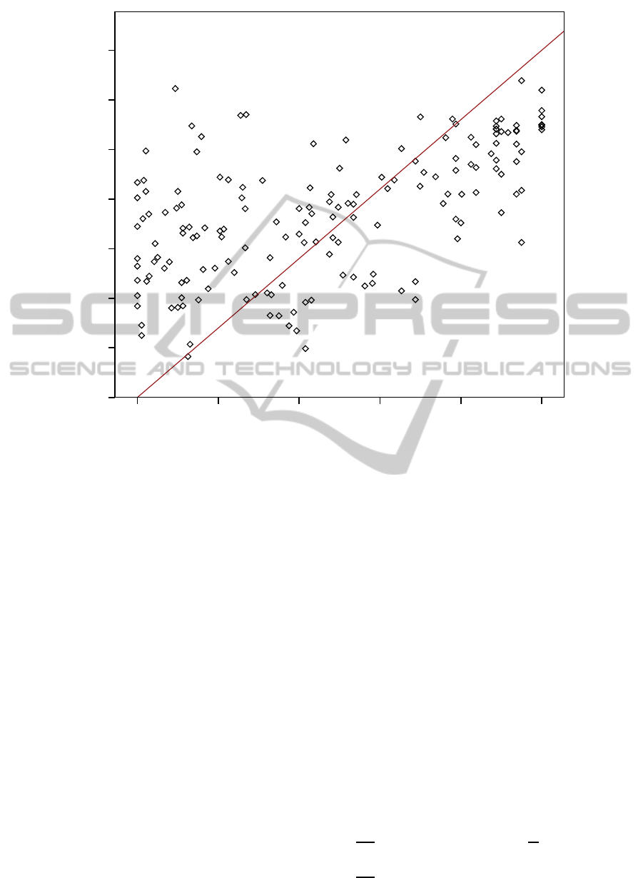
in scatter plots like in Figure 1.

Having longitudinal data allows to estimate

various sophisticated panel regression models

(Wooldridge, 2010). The most common ones are

ﬁxed effect (Allison, 2005) and random effect

SIMULTECH2013-3rdInternationalConferenceonSimulationandModelingMethodologies,Technologiesand

Applications

128

Democracy

1.00.80.60.40.20.00

log GDP per capita

12.00

11.00

10.00

9.00

8.00

7.00

6.00

5.00

2006

Quatar

United Arab

Emirates

Kuwait

Bahrain

Saudi

Arabia

Oman

Lybia

Zimbabwe

Myanmar

Morocco

Mexico

Liechtenstein

Norway

Mali

Liberia

Sierra Leone

Namibia

Nicaragua

Sao Tome

Congo

Kiribati

USA

Greece

South Korea

Bulgaria

Botswana

Kazachstan

Israel

Slovakia

Costa Rica

Poland

Vanautu

Kenya

Figure 1: The ﬁgure shows a correlation scatter plot for GDP per capita and democracy in the year 2006 for 189 countries. The

democracy index is based on Freedom House civil and political rights scores weighted for the actual human rights situation

(based on Cingranelli/Richards Human Rights data project) in the respective countries (Welzel, 2013). Most of the outliers at

the bottom right are oil-rich Middle East countries with high GDP but low democracy levels.

models (Laird and Ware, 1982). In these regression

analyses lagged or difference variables are used

as dependent variables to predict the value or the

difference of the independent variable at some later

point in time (Wooldridge, 2010). Autoregressive

(ibid.), two-stage least-square (Garson, 2013) and

simultaneous equation models (Wooldridge, 2010)

are further elaborated model speciﬁcations. There are

also non-linear versions panel regression models, like

logit regression models (ibid.).

In the analysis of GDP per capita and democracy

Barro (1996, 1999) used for instance a panel regres-

sion models with roughly 100 countries between 1960

and 1990 with GDP growth rates (difference vari-

ables) over three periods (1965-75), (1975-85) and

(1985-90) as dependent variables in an instrumen-

tal variable estimation approach with amongst others

democracy as predictor. He also computed regres-

sion models with average democracy levels (1965-

74),(1975-84) and (1985-94) with amongst others

lagged GDP levels as predictors. Performing these

panel analysis, Barro concludes that while democ-

racy has no signiﬁcant direct effect on GDP per capita

growth, GDP per capita has a signiﬁcant positive ef-

fect on democracy (Barro, 1996).

As suggested by Figure 2 there is a general linear

growing tend for both GDP and democracy. How-

ever, from this general trend it is difﬁcult to make any

reasonable conclusions about the dynamical interac-

tion of economy and democracy. More recent analy-

sis (Boix and Stokes, 2003; Krieckhaus, 2003) indeed

suggest that the relation between GDP and democracy

might be rather a non-linear and dynamic one. When

we create a phase portrait for GDP and democracy

the non-linearity and dynamics of their interaction be-

comes clear (see Figure 3).

Our analysis approach with data from 1980 to

2006 would result in these two best-ﬁt mathematical

models for democracy’s change as a function of GDP

and democracy itself and for GDP’s change as a func-

tion of democracy and GDP itself:

= 0.0003G

− 0.4031

(5)

= 0.0246D+ 0.0017G− 0.0002G

(6)

ABayesianApproachtoModelingDynamicalSystemsintheSocialSciences

129

year

2005

2003

2001

1999

1997

1995

1993

1991

1989

1987

1985

1983

1981

Value

1.2

1.0

0.8

0.6

0.4

0.2

Democracy

GDP(rescaled)

Figure 2: Sequence chart with average (all countries) rescaled GDP and average (all countries) democracy in a time line

between 1981 and 2006.

0 0.1 0.2 0.3 0.4 0.5 0.6 0.7 0.8 0.9 1

Democracy

GDP

Italia

Sweden

India

Chile

Albania

Nigeria

Figure 3: Visualisation of a phase portrait: changes in democracy values (x-axis) against log GDP (y-axis). The vector ﬁeld

shows average change according to the model, while the coloured lines give changes in representative countries as predicted

by the model given initial conditions in 1980. Speciﬁcally, the ODE model is integrated forward to 2006 for each country

starting with the actual initial condition for the corresponding country in 1980. The democracy index is based on Freedom

House civil and political rights scores weighted for the actual human rights situation (based on Cingranelli/Richards Human

Rights data project) in the respective countries.

The symbiotic interaction of these two variables,

economy and democracy, produces an interesting de-

velopment pattern in the phase-portrait ﬁgure (see

Figure 3). It seems countries typically head towards,

what in dynamical systems is called, a stable man-

ifold. Countries begin either side of this manifold,

some with high democracy and low GDP, others with

low democracy and high GDP. Over time the coun-

tries move to a common trajectory moving from bot-

tom left to top right of the phase plane. These results

can explain the sometimes apparently contradictory

patterns previously seen in relating GDP and democ-

racy. If a country starts with high democratic levels

but a GDP that is rather low, the democratic level is

unstable and regresses to the point where it reaches

the stable manifold that then allows both democracy

and GDP to grow again.

4 CONCLUSIONS

Our method provides social scientists with a tool to

study complex and dynamic phenomena. Unlike clas-

sic panel analysis, where a decision is usually made

to study a particular time frame, our methods takes in

to account all of the available temporal data. In the

application example, we are able to capture dynami-

cal interplays of variables. We expect that the method

will be able to detect more complex phenomena, such

as ampliﬁcation, growth limitation, glacial effects or

SIMULTECH2013-3rdInternationalConferenceonSimulationandModelingMethodologies,Technologiesand

Applications

130

tipping effects. The analysis procedure results in best-

ﬁt models that explicitly depict precise and dynamic

mechanisms. Equations such as 5 and 6 provide the

researcher with rich information beyond correlation

coefﬁcients, since they express how variables change

with respect to each other’s state. In future studies, we

will show how the same mechanisms can be used to

look at three and more variables(Ranganathan et al.,

2013).

A key feature of our approach is that no prede-

ﬁned model is imposed on the data. Instead the data

itself is used to ﬁnd the best model. The same ap-

proach of calculating Bayes factor can of course be

used to test theoretically informed model speciﬁca-

tions. Such testing can tell us how the best ﬁt data-

driven model compares in terms of statistical ﬁt, to

a model based on theoretical reasoning. There may

well be strong grounds to accept a theoretically jus-

tiﬁed model with a slightly worse ﬁt, over a purely

data-driven model with the best ﬁt. Indeed, we do not

suggest that social scientists should forget about the-

ories and always adopt the statistically best models.

No doubt, theories are useful to interpret results and

to evaluate models. But we think that social scientists

should be equally open to ﬁnding meaningful patterns

and mechanisms beyond established theories. If the

detected patterns and models are plausible and help to

understand social reality or give a new insight into a

phenomenon, then even new theoretical mechanisms

could be formulated or older theoretical mechanisms

revised, based on these ﬁndings.

REFERENCES

Allison, P. (2005). Fixed Effects Regression Methods for

Longitudinal Data. SAS Publishing.

Amemiya, T. (1985). Advanced econometrics. Blackwell,

Oxford.

Andersen, R. (2007). Modern Methods for Robust Regres-

sion. SAGE, London.

Ashimov, A. A., Sultanov, B. T., Adilov, Z. M., Borovskiy,

Y. V., Novikov, D. A., Nizhegorodtsev, R. M., and

Ashimov, A. A. (2011). Macroevonomic Analysis

and Economic Policy Based on Parametric Control.

Springer.

Barro, R. J. (1996). Democracy and growth. Journal of

Economic Growth, 1.

Barro, R. J. (1999). Determinants of democracy. Journal of

Political Economy, 107.

Bishop, C. M. (2006). Pattern recognition and machine

learning. Springer.

Boix, C. and Stokes, S. (2003). Endogenous democratisa-

tion. World Politics, 55.

Coleman, J. S. (1964). Introduction to Mathematical Soci-

ology. Free Press of Glencoe/Collier Macmillan.

de Marchi, S. (2005). Computation and Mathematical Mod-

eling in the Social Sciences. Cambridge University

Press.

Diamond, L. and Marks, G. (1992). Reexamining Democ-

racy. SAGE.

Garson, G. D. (2013). Two-Stage Least Square Regression.

Statistical Associates Publishers.

Gelman, A. (2004). Exploratory data analysis for com-

plex models. Journal of Computational and Graph-

ical Statistics, 13 (4).

Krieckhaus, J. (2003). The regime debate revisited: A sensi-

tive analysis of democracy’s economic effect. British

Journal of Political Science, 34.

Laird, N. M. and Ware, J. H. (1982). Random-effects mod-

els for longitudinal data. Biometrics, 38 (4).

Lewis-Beck, M. S. (1995). Data Analysis: An Introduction.

SAGE, London.

Ley, E. and Steel, M. F. (2009). On the effect of prior as-

sumptions in bayesian model averaging with applica-

tions to growth regression. Journal of Applied Econo-

metrics, 24:651–674.

Lipset, S. M. (1959). Some social requisites of democ-

racy: Economic development and political legitimacy.

American Political Science Review, 53.

Menard, S. (2001). Applied Logistic Regression Analysis.

SAGE, London.

Ostrom, C. W. (1990). Time Series Analysis: Regression

Techniques. SAGE, London.

Ranganathan, S., Mann, R. P., Nikolis, S. C., Swain, R. B.,

and Sumpter, D. J. (2013). A dynamical systems ap-

proach to modeling human development. Economet-

rica. submitted.

Robert, C. P. (1994). The Bayesian Choice: a decision-

theoretic motivation. Springer-Verlag, New York.

Saperstein, A. M. (2000). Dynamical Modeling of the Onset

of War. World Scientiﬁc Publishing Company.

Stebbins, R. A. (2001). Exploratory Research in Social Sci-

ences. SAGE, London.

Strogatz, S. H. (2000). Nonlinear Dynamics and Chaos:

With Applications to Physics, Biology, Chemistry and

Engineering. Westview Press.

Treiman, D. L. (2009). Quantitative Data Analysis: Doing

Social Research to Test Ideas. Jossey-Bass.

Tukey, J. (1977). Exploratory Data Analysis. Addison-

Wesley.

Weber, L. (2012). Demographic Change and Economic

Growth: Simulation on Growth Modeling. Physica.

Welzel, C. (2013). Freedom Rising. Human Empowerment

and the Quest for Emancipation. Cambridge Univer-

sity Press.

Wooldridge, J. M. (2010). Econometric Analysis of cross

section and panel data. MIT Press.

ABayesianApproachtoModelingDynamicalSystemsintheSocialSciences

131