
Towards an EDSL to Enhance Good Modelling Practice for Non-linear
Stochastic Discrete Dynamical Models
Application to Plant Growth Models
Benoit Bayol, Yuting Chen and Paul-Henry Cournède
Ecole Centrale Paris, Laboratory of Applied Mathematics and Systems, 92290, Châtenay-Malabry, France
Keywords:
General State-space Model, Grid Simulation, Parallelism, Parameter Estimation, Filtering, Sensitivity
Analysis, Uncertainty Analysis, Model Selection, Data Assimilation, Multi-paradigm Programming, EDSL.
Abstract:
A computational formalism is presented that structures a C++ library which aims at the modelling, simulation
and statistical analysis of stochastic non-linear discrete dynamical system models. Applications concern the
development and analysis of general plant growth models.
1 INTRODUCTION
With the increasing need in modelling in all fields of
science, and sometimes a lack of precautions in the
way models are developed and used, some authors
tried to define and promote good modelling practices
for environmental sciences (Van Waveren et al., 1999)
or in physiology and medicine (Carson and Cobelli,
2001) by proposing different steps in the modelling
process, from conceptual work to model applications.
These steps include the use of statistical analysis tools
like parameter estimation, sensitivity analysis, uncer-
tainty analysis or model selection.
Some existing numerical platforms like R, Scilab
or Matlab propose existing algorithms belonging to
these categories but no real standardization for the
inputs and outputs of these tools. Moreover some
existing modelling platforms like Modelica, Xcos or
Simulink have a good modelling framework but are
mainly deterministic and stream oriented which pre-
vents implementing powerful estimation methods in
a proper statistical framework. Finally all these plat-
forms are disconnected in the sense that going from
one to another for analyzing a model is not an easy
task in terms of engineering. Each tools and algo-
rithms have a different set of required inputs.
In this context, our objective is to design a single
library that allows to create, to evaluate and to ana-
lyze models with a common language among mod-
ellers and statisticians. This library has the following
characteristics :
• it uses a multi-paradigm programming style with
emphasis on generic and functional paradigms.
• it uses a common syntax for modelling, simula-
tion and analysis algorithms.
• it provides a flexible template for model observa-
tions, adapted to the heterogeneous and irregular
observations of biological systems.
• it is adapted to stochastic systems, particularly
the implementation of modelling and observations
noises.
• implements statistical methods for model analysis
and evaluation
In section 2, we describe the modellingframework
of the platform. In section 3, we show how to repre-
sent the simulation framework with a projection on a
3D-grid that eases the implementation of numerical
methods and their parallel computation. In section 4,
we present an overview of the implemented methods.
In section 5, we illustrate the potentials of the library
on a complex test case of data assimilation of a plant
model. Finally, we will discuss about the perspectives
of this library.
2 MODELLING
Better understanding of plant development and
growth is a key issue to make agriculture practice
more competitive and more respectful of the environ-
ment.
Agronomic researchers and engineers have built
several models for this purpose. Geometrical or em-
132
Bayol B., Chen Y. and Cournède P..
Towards an EDSL to Enhance Good Modelling Practice for Non-linear Stochastic Discrete Dynamical Models - Application to Plant Growth Models.
DOI: 10.5220/0004481101320138
In Proceedings of the 3rd International Conference on Simulation and Modeling Methodologies, Technologies and Applications (SIMULTECH-2013),
pages 132-138
ISBN: 978-989-8565-69-3
Copyright
c
2013 SCITEPRESS (Science and Technology Publications, Lda.)

pirical at first, models are more and more mechanistic,
with the development of agro-environmental ((Bris-
son et al., 2003)), and functional-structural models
((de Reffye et al., 2008), (Vos et al., 2010)) which
are used for the description at macro and mesoscale
levels.
These mechanistic models have the following
characteristics:
• complexity in terms of the numbers of interacting
processes and of parameters.
• difficult parameter estimation due to the non-
linearity of the model and irregularity of data.
• sophisticated and costly methods for their analy-
sis.
• possibly high memory need during computation
for models of plants with complex structures like
trees.
A general representation of plant growth can be
given in the general state-space form, with model
equations describing the discrete evolutionof the state
variables X ∈ R
x
across time steps, and observation
equations, giving the system observation variables
X ∈ R
y
as functions of the state variables (Cournède
et al., 2011). For biological systems, these observa-
tion functions may be very rare (no observation at
most time steps) and heterogeneous (different types
of observations at different observation times).
Let us decompose the observation vectors Y in k
elementary sub-vectors Y = (Y
1
,Y
2
, . . . ,Y
k
), such that
at each step of system observation j, the observa-
tion function G
j
can be described by a subset of the
{Y
i
}
1≤i≤k
, corresponding to the set of variables that
are observed at step j. The elementary sub-vectors Y
i
are called observers (their choice is not unique) and
τ
i
= { j such that Y
i
is observed at step j} is called the
timeline of observer i.
Equation (1) describes the general state-space
form taking into account the irregularity and hetero-
geneity of data.
X
n+1
= F
n
(X
n
,U
n
, P, ε
n
)
Y
n
= G
n
(X
n
, P, ε
′
n
) = (Y
i
Λ
τ
i
(n))
1≤i≤k
(1)
with Λ
τ
i
(n) = 1 if n ∈ τ
i
, else 0.
In order to translate Equation (1) into an effective
code for simulation, we first give the following defi-
nitions:
• A dynamical model denotes a 6-tuple M =
{X,U, P, ε
M
, INIT, NEXT} where:
– {X,U, P} denote respectively the set of state
variables, the set of control variables, the set
of parameters of the full model.
– ε
M
denotes the set of stochastic variables of
the model errors. The space dimension corre-
sponds to the dimension of the random vector
used in the model equations.
– INIT denotes an initialization function to deter-
mine the initial state X
0
such as X
0
= INIT(P)
and INIT : X × P → X
– NEXT represents the transition function of the
dynamical model such as NEXT : X ×U × P×
ε
M
→ X
• An observation model denotes a 5-tuple O =
{X, P,Y, ε
O
, OBSERVE} where:
– Y denotes the output of the observation model.
– ε
O
denotes the set of stochastic variables for the
observation errors.
– OBSERVE denotes an observation function
such as OBSERVE : X × P× ε
O
→ Y
• An observer denotes a 2-tuple O = {O, TML}
where TML is a timeline which controls the ob-
servation of the dynamical system.
Thus the global stochastic dynamic
system model (with observations) is de-
noted by a 8-tuple S = {X,U, P,Y, ε
M
+
{ε
O
}
1≤i≤k
, INIT, NEXT, {OBSERVE, TML}
1≤i≤k
}
where:
• the indexes i, 1 ≤ i ≤ k represent different ob-
servers. We do not consider a unique observer be-
cause of the irregularity and diversity of observed
variables. It is a very important specificity of bi-
ological systems for which experiments are diffi-
cult or costly (Cournède et al., 2011). The error
models for each observer will also be specific.
• ε
M
+{ε
O
}
1≤i≤k
represents the total set of stochas-
tic vectors for model simulation.
To generate the random sequences (ε
n
)
0≤n≤N− 1
∈
(ε
M
)
N
, with N the maximum simulation time and
(ε
′
n
)
0≤n≤N− 1
∈ (ε
O
)
N
, for each of the k different ob-
servers, we also define a random vector model by a
3-tuple V = {P, ε
V
, LAW} such as:
• P denotes the set of parameters of the LAW.
• ε
V
is the set of stochastic vectors
• LAW represents the law of the probability distribu-
tion such as LAW : P×[0;1]
v
→ ε
V
, where v is the
dimension of the random vector: if ε
V
⊂ R
v
is a
probability space of dimension v, there exists a bi-
jection ψ from [0;1]
v
onto ε
V
given by the inverse
of the marginal cumulative distribution function
of each component.
TowardsanEDSLtoEnhanceGoodModellingPracticeforNon-linearStochasticDiscreteDynamicalModels-
ApplicationtoPlantGrowthModels
133
A simulation of the random vector is thus built
from a random model V and a generator that gen-
erates a sequence in [0;1]
v
. Different types of gen-
erators exist (pseudo-random based on congruential
sequences for example as Mersenne-Twister (Mat-
sumoto and Nishimura, 1998), quasi-random (Ko-
cis and Whiten, 1997), ...). The sequence generated
by the generator is usually uniquely determined by
a seed, corresponding to the first element of the se-
quence in [0;1]
v
. Therefore, a simulation of the ran-
dom vector is a 5-tuple {V , p, N, S
0
, GENERATE}
where S
0
is the seed of generator and GENERATE
the function that generate the random sequence in
[0;1]
v
, p ∈ P and N the maximal time of the simu-
lation.
Such random variable simulation is used in the
dynamical system simulation to generate both model
and observation noises (for each of the k observers).
3 SIMULATION
In this section we detail how the modelling frame-
work can be projected onto a ’simulation grid’ to cate-
gorize and formalize the different algorithms used for
model analysis. This also helps to consider the tran-
sition to parallel computing. The categorization will
be conducted both in terms of input arguments of the
algorithms and pathways.
We give the following definitions:
• a context c denotes the initial conditions and as-
sociated control variables. In our case, the control
variables are given by the environmental condi-
tions and are supposed to be fully known at the
beginning of the simulation. Therefore c is com-
posed of X
0
and (U
n
)
0≤n≤N
, where N represents
the last time step of the simulation.
• parameters p are the full vector of parameters of
the observation model and dynamical model.
• an observer list [o] denotes the composition of
several observers i.e. a several observation func-
tions with their timelines.
• a list of seed [seed] is given to either dynamical
model or observation model for initializing the
random generators.
• an observation list y denotes the result of ob-
servers during a simulation
• a simulation is the combination of a dynamical
model, an observer list, a context and a set of pa-
rameters
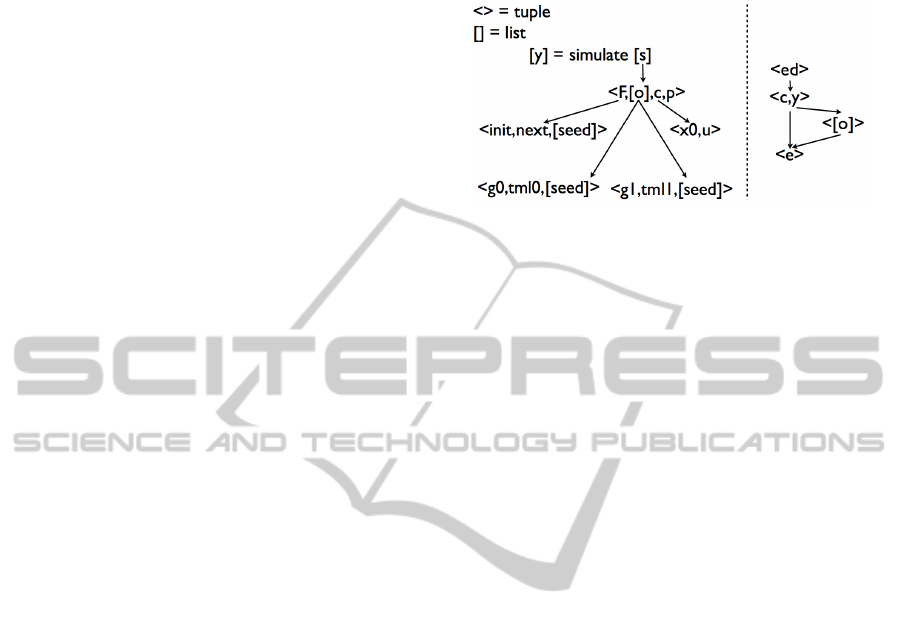
• simulate denotes a function that applies a param-
eters set to a list of simulations.
Left of the figure 1 summarizes all these concepts in
a syntax tree.
Figure 1: Simulation syntax tree.
Moreover a key feature for interacting with users
is to rebuild simulations from experimental data by
extracting the list of context and observer list. For
this purpose we define:
• an experimental data ed denotes data that have
been observed for a given context.
• experiment e denotes observations that will be ob-
served for a given context. Experiment is a tuple
composed of a context and an observer list.
Right of the figure 1 summarizes these two concepts.
us defined data structures for representing obser-
vation data and simulations, and a simulation func-
tion.
As we will see in section 4 most algorithms use a
combination of contexts and parameters as inputs. As
a result, these algorithms manipulate lists of simula-
tion.
A conceptual grid helps to classify the algorithms
of interest for model analysis and estimation detailed
in section 4. The classification is done regarding
which part of the grid is used and how we go through
it.
For the sake of clarity, we leave aside the notion
of observer and use only context and parameters.
Algorithms in section 4 have to simulate a list of
simulations by the combination of:
• a lot of contexts for a given parameter set.
• a single context with a lot of parameter sets.
• a lot of contexts with a lot of parameter sets.
On figure 2 we give a representation of the simulation
grid, with the following axis:
• x-axis for contexts.
• y-axis for parameter sets.
• z-axis for time steps.
For each triple (x, y, z) we associate an equivalent
triple (C
i
, P
j
, n) and its transformation [Y
n
]
j
i
through
SIMULTECH2013-3rdInternationalConferenceonSimulationandModelingMethodologies,Technologiesand
Applications
134

Figure 2: Grid for simulation.
the simulation function which is the result of doing
observations at time n on cell (i, j).
There are two ways for going through the grid:
• in one single run which corresponds to obtaining
a full observation vector for all simulations.
• per step which corresponds to obtaining a slice of
observations as shown in figure 2.
Both model and observation equations might be
perturbed by noises. There is a unique random gener-
ator for each noise, that is to say for each stochastic
variable.
In figure 2 each cell of the plane (corresponding to
one context and one parameter set) has its own gen-
erator list denoted by a black dot. This black point is
composed of several dots which are the seed of each
random generator. ∼ { ε
M
} is the generator associated
to the model noises and ∼ {(ε
O
)
i
} is the generator as-
sociated to the observer O
i
, for all i, 1 ≤ i ≤ k. The
curves illustrate the random trajectories.
4 ANALYSIS
Key steps in the modelling process concern analysis
and parameter estimation.
The following methods are implemented in the
platform:
• Frequentist Parameter Estimation Ap-
proaches, like generalized least squares estimator
(GLSE) or maximum likelihood estimator
(MLE). Generally, the estimation involves a
context list and an observer list, and handles
at each algorithmic step a single parameter
set. It is not the case however, for Monte-
Carlo methods such as stochastic expectation-
maximization (see (Trevezas and Cournède,
2013) in the context of plant growth). The
equivalent function signature with previous no-
tations is frequentist_parameter_estimation(<
M, [ed], p >). We only go through the first row
of the grid to compute all observation lists [Y]
i
0
with only one parameter set. Then we compare
all these lists to the experimental one and select
another parameter set to minimize this distance.
• Bayesian Inference Approaches based on Fil-
tering Methods, like convolution particle filter
(Chen and Cournède, 2012) or unscented kalman
filter (Julier et al., 2000), take a single con-
text and an observer list with a list of param-
eter sets. The equivalent function signature is
filtering_parameter_estimation(< M, ed, [p] >
). We only go through the first column of the grid
and stop at each observation time step to imple-
ment the filtering process based on the experimen-
tal data: at each observation step, the parameters
and states are updated for all the selected simula-
tions. The idea is to provide estimations with re-
liable uncertainty that are appropriately assessed
with the population of parameter sets. A more
detailed presentation of convolution particle filter
can be found in 5.
• Sensitivity Analysis Approaches, like standard
regression coefficient or Sobol (Saltelli et al.,
2008) (Wu et al., 2012), take a single context and
an observer list with a list of parameter sets. The
equivalent function signature with previous no-
tation is sensitivity_analysis(< M, e, [p] >). The
way of going trough the grid is slightly the same
as for filtering parameter estimation methods. The
exception concerns the different triggers. In sensi-
tivity analysis parameters are not changed during
the algorithm.
• Uncertainty Analysis Approaches, using Monte
Carlo samples or the unscented transform (Julier
et al., 2000), follow the same rules as sensitiv-
ity analysis. The equivalent function signature is
uncertainty_analysis(< M, e, [p] >).
• Model Selection (Baey et al., 2012) computes cri-
terion like mean square prediction error or Akaike
information criterion for a list of models. A cri-
terion follows the signature model_selection(<
M, [ed], p >) but the general method will use a list
of models [M] for making comparison among the
criterion results.
5 TEST CASE
In this section we describe the context of convolu-
tion particle filtering and its characteristics. Previous
elements are not specifically related to plant growth
TowardsanEDSLtoEnhanceGoodModellingPracticeforNon-linearStochasticDiscreteDynamicalModels-
ApplicationtoPlantGrowthModels
135
models. In this test case, we consider the param esti-
mation of a plant growth model. Some specific char-
acteristics have to be taken in account.
As said in section 1 plant growth models are gen-
erally characterized by complex interacting processes
and a great number of model parameters. Moreover
experimental data acquisition tends to be costly (ex-
periments in fields), inaccurate (coming from satel-
lite images), and irregular (sometimes observations
can not be done). Thus the parametrization of these
models is a key issue which may affect the quality of
model prediction. Therefore we use the convolution
particle filter method. (Campillo and Rossi, 2009) and
an adaptation developed by (Chen et al., 2012).
The objective of this method is to estimate jointly
the parameters and the hidden states of the system
from online data i.e. data that comes from time to
time improving the database. This kind of technique
is known as data assimilation. The idea is to sam-
ple M particles (i.e. a parameter set and a state) and
to propagate them through the model until the next
available measurement to compare with the predicted
states. Then we compute for each particle a weight,
according to experimental data and prediction, which
helps to classify and select the best particles that are
closer to the real experimental case.
The following results are based on the CPF
method applied to the Log Normal Allocation and
Senescence (LNAS) daily crop model with real ex-
perimental data (Chen et al., 2013). The equations
of the LNAS model are derived for sugar beet with
three main processes during the plant growth period:
biomass production, allocation and senescence. Two
compartments are taken into account: foliage and root
system.
Based on the parameter estimation results from
the 2010 dataset with an iterative version of the CPF
method, we conducted the data assimilation approach
with the CPF algorithm by recalibration the parame-
ters and readjusting the hidden states of interest based
on the data of early growth stage (five first data) of the
2006 dataset. The predictive capacity of the model
for the last two dates of measurements is compared
in two cases: with data assimilation and from pure
uncertainty analysis (based on the calibration result,
propagation of the uncertainty with the 2006 context).
In our example we consider data col-
lected at 12 different dates in 2010
for the calibration step: O
2010
=
{54, 68, 76, 83, 98, 104, 110, 118, 125, 132, 145, 160}.
We also have 7 measurement dates in 2006:
O
2006
= {54, 59, 66, 88, 114, 142, 198}
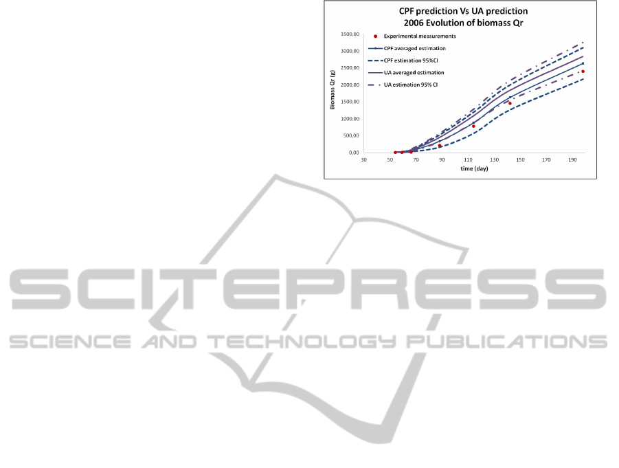
Figure 3 illustrates the prediction results given by
the two cases. In the case of data assimilation with
Figure 3: Comparison of CPF Data Assimilation with
Monte Carlo UA method.
CPF, not only the point predictions are more accu-
rate, but the related uncertainty is also reduced. On
the contrary, the predicted confidence interval given
by uncertainty analysis (without data assimilation)
does not even contain the real measurements (last two
points). This result clearly suggests an obvious ad-
vantage of the CPF data assimilation method in terms
of prediction capacity.
However such method is rather time and memory
consuming since for a run with 40 000 particles we
need 8 Gb of RAM and 18 hours of computation for
a sequential job. The advantage and feasibility of par-
allel computation is obvious with the formalization as
a simulation grid, and we are currently working on
the implementation. Of course, the computation time
depends also of the analyzed model.
6 DISCUSSION
We have shown the basic principles that structure our
library and how they are related to the domain of ap-
plication, discrete nonlinear, stochastic models, with
potentially heterogeneous or rare observations, with
the example of plant growth. There are still some
steps to fulfill in order to call it a domain-specific lan-
guage.
6.1 Towards an embedded Domain
Specific Language
An embedded domain specific language is a language
hosted into another one with a semantic dedicated
to a domain. It has the characteristic to exploit the
host language syntax which helps to focus on domain-
specific question and reduce maintenance.
The choice of C++ has been made in regards of:
• developers skills inside the project
SIMULTECH2013-3rdInternationalConferenceonSimulationandModelingMethodologies,Technologiesand
Applications
136

• the number of reliable libraries in the community
like Boost, MKL or Armadillo
• the philosophy of "abstractions that do not impose
space or time overheads" (Stroustrup, 2012)
• its performance compared to other existing lan-
guages (Hundt, 2011)
Our current work is to formalize the ideas that
have been developed in section 2 and section 3 by
defining the abstract syntax tree and inference rules.
Genericity of the library is an important goal, es-
pecially the ability to analyze any model that can be
formulated by equation 1.
We use templates because of its capacity of em-
ulating structural sub-typing and by experience this
kind of sub-typing is more convenient to our activity
than nominal sub-typing with the original inheritance
mechanism of object-oriented programming. More-
over this orientation could allow us to use structures
or tuples in conjunction with Vexcl or Thrust libraries
in an easy way through tag dispatching technique.
6.2 Workflow
This framework was built with constant exchanges
between the modellers, the mathematicians develop-
ing the methods, and software engineers. It helped us
to understand the domain of course but also the way
we were working on this domain. Most of the time a
given model is associated to a given modeller and the
transmission and integration in terms of code is quite
complex if it does not follow a strict interface. There-
fore we have defined a terminology and tool for man-
aging this workflow. The tool is developed in python
and is inspired by management tool frequently avail-
able with web framework like Rails or Symfony. The
platform itself cannot be seen without its managing
tool in order to establish a way of communication dur-
ing the development of models and methods.
6.3 Conclusions
The above formalism has been designed with a
bottom-up approach and is used in our team for the
implementation of our tools. It unifies our thinking
about modelling, simulation and analysis.
We did not linked yet our work to existing for-
malism like DEVS, stochastic petri nets, P-DEVS, pi-
calculus. We expect to find a way for the support
of concurrency models for biological systems like
plant-soil interaction by looking at DEVS/P-DEVS
and DESS. (Zeigler et al., 1995)
In the long term we believe that that a DSL can be
derived from our EDSL for delivering a GUI tool to
end-users.
REFERENCES
Baey, C., Didier, A., Li, S., Lemaire, S., Maupas, F., and
Cournède, P.-H. (2012). Evaluation of the Predictive
Capacity of Five Plant Growth Models for Sugar Beet.
In Kang, M., Dumont, Y., and Guo, Y., editors, Plant
Growth Modeling, Simulation, Visualization and Ap-
plications - PMA12, pages 30–37, Shanghai, China.
IEEE.
Brisson, N., Gary, C., Justes, E., Roche, R., Mary, B.,
Ripoche, D., Zimmer, D., Sierra, J., Bertuzzi, P.,
Burger, P., Bussiére, F., Cabidoche, Y., Cellier, P.,
Debaeke, P., Gaudillére, J., Hènault, C., Maraux, F.,
Seguin, B., and Sinoquet, H. (2003). An overview of
the crop model STICS. European Journal of Agron-
omy, 18:309–332.
Campillo, F. and Rossi, V. (2009). Convolution Particle Fil-
ter for Parameter Estimation in General State-Space
Models. IEEE Transactions in Aerospace and Elec-
tronics., 45(3):1063–1072.
Carson, E. and Cobelli, C. (2001). Modelling Methodology
for Physiology and Medicine. Academic Press, San
Diego (US).
Chen, Y., Bayol, B., Loi, C., Trevezas, S., and Cournède, P.-
H. (2012). Filtrage par noyaux de convolution itératif.
In Actes des 44émes Journèes de Statistique JDS2012,
Bruxelles 21-25 Mai 2012.
Chen, Y. and Cournède, P.-H.(2012). Assessment of param-
eter uncertainty in plant growth model identification.
In Kang, M., Dumont, Y., and Guo, Y., editors, Plant
growth Modeling, simulation, visualization and their
Applications (PMA12). IEEE Computer Society (Los
Alamitos, California).
Chen, Y., Trevezas, S., and Cournède, P.-H. (2013). Itera-
tive convolution particle filtering for nonlinear param-
eter estimation and data assimilation with application
to crop yield prediction. In Society for Industrial and
Applied Mathematics (SIAM): Control & its Applica-
tions,San Diego, USA.
Cournède, P.-H., Letort, V., Mathieu, A., Kang, M.-Z.,
Lemaire, S., Trevezas, S., Houllier, F., and de Reffye,
P. (2011). Some parameter estimation issues in
functional-structural plant modelling. Mathematical
Modelling of Natural Phenomena, 6(2):133–159.
de Reffye, P., Heuvelink, E., Barthélémy, D., and Cournède,
P.-H. (2008). Plant growth models. In Jorgensen, S.
and Fath, B., editors, Ecological Models. Vol. 4 of En-
cyclopedia of Ecology (5 volumes), pages 2824–2837.
Elsevier, Oxford.
Hundt, R. (2011). Loop recognition in c++/java/go/scala.
In Proceedings of Scala Days 2011.
Julier, S., Uhlmann, J., and Durrant-Whyte, H. (2000). A
new method for the nonlinear transformation of means
and covariances in filters and estimators. IEEE Trans-
actions on Automatic Control, 45(3):477–482.
Kocis, L. and Whiten, W. J. (1997). Computational inves-
tigations of low-discrepancy sequences. ACM Trans.
Math. Softw., 23(2):266–294.
Matsumoto, M. and Nishimura, T. (1998). Mersenne
twister: a 623-dimensionally equidistributed uni-
form pseudo-random number generator. ACM Trans.
Model. Comput. Simul., 8(1):3–30.
TowardsanEDSLtoEnhanceGoodModellingPracticeforNon-linearStochasticDiscreteDynamicalModels-
ApplicationtoPlantGrowthModels
137

Saltelli, A., Ratto, M., Andres, T., Campolongo, F., Cari-
boni, J., Gatelli, D., Saisana, M., and Tarantola,
S. (2008). Global Sensitivity Analysis. John Wi-
ley&Sons, the primer edition.
Stroustrup, B. (2012). Foundations of c++. In Seidl, H.,
editor, Programming Languages and Systems, volume
7211 of Lecture Notes in Computer Science, pages 1–
25. Springer Berlin Heidelberg.
Trevezas, S. and Cournède, P.-H. (2013). A sequential
monte carlo approach for mle in a plant growth model.
Journal of Agricultural, Biological, and Environmen-
tal Statistics, In press.
Van Waveren, R., Groot, S., Scholten, H., Van Geer, F.,
Wosten, H., Koeze, R., and Noort, J. (1999). Good
modelling practice handbook. Technical Report 99-
05, STOWA, Utrecht, RWS-RIZA, Lelystad, The
Netherlands.
Vos, J., Evers, J. B., Buck-Sorlin, G. H., Andrieu, B.,
Chelle, M., and de Visser, P. H. B. (2010). Functional-
structural plant modelling: a new versatile tool in crop
science. Journal of Experimental Botany, 61(8):2101–
2115.
Wu, Q., Cournède, P.-H., and Mathieu, A. (2012). An
efficient computational method for global sensitivity
analysis and its application to tree growth modelling.
Reliability Engineering & System Safety, 107:35–43.
Zeigler, B., Song, H. S., Kim, T. G., and Praehofer, H.
(1995). Devs framework for modelling, simulation,
analysis, and design of hybrid systems. In In Proceed-
ings of HSAC, pages 529–551. Springer-Verlag.
SIMULTECH2013-3rdInternationalConferenceonSimulationandModelingMethodologies,Technologiesand
Applications
138
