
Computational Experience in Solving Continuous-time Algebraic Riccati
Equations using Standard and Modified Newton’s Method
Vasile Sima
Advanced Research, National Institute for Research & Development in Informatics,
Bd. Mares¸al Averescu, Nr. 8–10, Bucharest, Romania
Keywords:
Algebraic Riccati Equation, Numerical Methods, Optimal Control, Optimal Estimation.
Abstract:
Improved algorithms for solving continuous-time algebraic Riccati equations using Newton’s method with or
without line search are discussed. The basic theory and Newton’s algorithms are briefly presented. Algorith-
mic details the developed solvers are based on, the main computational steps (finding the Newton direction,
finding the Newton step size), and convergence tests are described. The main results of an extensive perfor-
mance investigation of the solvers based on Newton’s method are compared with those obtained using the
widely-used MATLAB solver. Randomly generated systems with orders till 2000, as well as the systems from
a large collection of examples, are considered. The numerical results often show significantly improved accu-
racy, measured in terms of normalized and relative residuals, and greater efficiency than the MATLAB solver.
The results strongly recommend the use of such algorithms, especially for improving the solutions computed
by other solvers.
1 INTRODUCTION
The numerical solution of algebraic Riccati equations
(AREs) is an essential step in many computational
methods for model reduction, filtering, and controller
design for linear control systems. Let A, E ∈ R
n×n
,
B ∈R
n×m
, and Q and R be symmetricmatrices of suit-
able dimensions. In a compact notation, the general-
ized continuous-time AREs (CAREs), with unknown
X = X
T
∈ R
n×n
, are defined by
0 = Q+ op(A)
T
X op(E) + op(E)
T
X op(A) (1)
−L(X)R
−1
L(X)
T
=: R (X),
where E and R are assumed to be nonsingular, and
L(X):=L+ op(E)
T
XB ,
with L of suitable size. The operator op(M) repre-
sents either M or M
T
. Define also G := BR
−1
B
T
. An
optimal regulator problem involves the solution of an
ARE with op(M) = M; an optimal estimator problem
involves the solution of an ARE with op(M) = M
T
,
input matrix B replaced (by duality) by the transpose
of the output matrix C ∈ R
p×n
, and m replaced by
p. (This means that L should be n× p in this case.)
In practice, often Q and L are given as C
T
¯
QC and
L = C
T
¯
L, respectively. The solutions of an ARE are
the matrices X = X
T
for which R (X) = 0. Usually,
what is needed is a stabilizing solution, X
s
, for which
the matrix pair (op(A − BK(X
s
)), op(E)) is stable
(in a continuous-time sense), where op(K(X
s
)) is the
gain matrix of the optimal regulator or estimator, and
K(X) := R
−1
L(X)
T
(2)
(with X replaced by X
s
).
There is a vast literature concerning AREs and
their use for solving optimal control and estimation
problems; see, e.g., the monographs (Anderson and
Moore, 1971; Mehrmann, 1991; Lancaster and Rod-
man, 1995) for many theoretical results. The op-
timization criterion for linear control systems is a
quadratic performance index in terms of the system
state and control input. By minimizing this criterion,
a solution to the optimal systems stabilization and
control is obtained, expressed as a state-feedback con-
trol law. Briefly speaking, this control law achieves a
trade-off between the regulation error and the control
effort. The optimal estimation or filtering problem,
for systems with Gaussian noise disturbances, can be
solved as a dual of an optimal controlproblem, and its
solution gives the minimum variance state estimate,
based on the system output. It is worth to say that the
results of an optimal design are often better suited in
practice than those found by other approaches. For
instance, pole assignment may deliver too large gain
5
Sima V..
Computational Experience in Solving Continuous-time Algebraic Riccati Equations using Standard and Modified Newton’s Method.
DOI: 10.5220/0004482500050016
In Proceedings of the 10th International Conference on Informatics in Control, Automation and Robotics (ICINCO-2013), pages 5-16
ISBN: 978-989-8565-70-9
Copyright
c
2013 SCITEPRESS (Science and Technology Publications, Lda.)

matrices, producing high-magnitude inputs, which
might not be acceptable. In both control and estima-
tion problems, including those stated in the H
∞
theory
(e.g., (Francis, 1987)), a major computational step is
the solution of an ARE. Due to their importance, nu-
merous numerical methods have been proposed for
solving AREs; see, for instance, (Mehrmann, 1991;
Sima, 1996). There are also several highly-used soft-
ware implementation, e.g., in MATLAB (MATLAB,
2011), or in the SLICOT Library (Benner et al., 1999;
Benner and Sima, 2003; Van Huffel et al., 2004; Ben-
ner et al., 2010).
Newton’s method for solving AREs has been con-
sidered by many authors, for instance, (Kleinman,
1968; Mehrmann, 1991; Lancaster and Rodman,
1995; Sima, 1996; Benner, 1997; Benner, 1998; Ben-
ner and Byers, 1998). Actually, the matrix sign func-
tion method for solving AREs, e.g., (Roberts, 1980;
Gardiner and Laub, 1986; Byers, 1987; Sima and
Benner, 2008), uses a specialized Newton’s method
to compute the square root of the identity matrix of
order 2n. This paper merely reports on implementa-
tion details and numerical results. In addition, there
are contributions compared to (Benner, 1998; Ben-
ner and Byers, 1998): improved stopping criteria, im-
proved functionality (regarding generality in the co-
efficient matrices and options), a better routine for
computing the roots of a third order polynomial, etc.
The paper extends the results of (Sima and Benner,
2006) in some details, and by investigating the nu-
merical behavior of the current Newton-based ARE
solvers for high-order random systems, and for sys-
tems from the COMPl
e
ib collection (Leibfritz and
Lipinski, 2003; Leibfritz and Lipinski, 2004). (The
previous paper (Sima and Benner, 2006) used ran-
domly generated systems with n ≤ 40, and systems
from the CAREX benchmark collection (Abels and
Benner, 1999), where most problems have small size,
but may be very ill-conditioned.) It is worth mention-
ing that Newton’s method has been applied in (Penzl,
2000) for solving special classes of large-orderAREs,
using low rank Cholesky factors of the solutions of
the Lyapunov equations built during the iterative pro-
cess (Penzl, 1998). Additional numerical results, for
randomly generated systems with n ≤ 600, and com-
parison with MATLAB and SLICOT solvers are pre-
sented in (Sima, 2005). However, contrary to stan-
dard solvers, the specialized solvers used (
lp lrnm
and
lp lrnm i
) are not general solvers. In order to
use them advantageously,the following main assump-
tions must be fulfilled: 1) the matrix A is structured or
sparse; 2) the solution X has a small rank in compar-
ison with n. (These solvers use the possibly sparse
structure of the matrix A and operations of the form
Ab or A
−1
b, where b is a vector.) The solvers dis-
cusssed in this paper are general, and can be used to
solve large dense problems.
The paper compares the performance of the New-
ton solver with or without line search with the per-
formance of the state-of-the-art commercial solver
care
from MATLAB Control System Toolbox. The
MATLAB solver uses a different, eigenvalue ap-
proach, based on the results in, e.g., (Laub, 1979;
Van Dooren, 1981; Arnold and Laub, 1984). Rela-
tively recent research, including both theoretical and
numerical investigation, has been directed to exploit
the Hamiltonian-symplectic structure of the eigen-
problem associated to the ARE (Raines and Watkins,
1992; Benner et al., 2002; Benner et al., 2007; Sima,
2010; Sima, 2011).
A recursive method for computing the positive
definite stabilizing solution of an ARE with an in-
definite quadratic term has been recently proposed
in (Lanzon et al., 2008).
One drawback of the Newton’s method is its de-
pendence on an initialization, X
0
. When searching for
a stabilizing solution X
s
, the initialization X
0
should
also be stabilizing, i.e., (op(A − BK(X
0
)), op(E) )
should be stable. Except for stable systems, finding a
suitable initialization can be a difficult task. Stabiliz-
ing algorithms have been proposed, mainly for stan-
dard systems, e.g., in (Kleinman, 1968; Varga, 1981;
Sima, 1981; Hammarling, 1982). However, often
these algorithms produce a matrix X
0
and/or the fol-
lowing several matrices X
i
, i = 1,2,... (computed by
the Newton method), with very large norms, and the
solver may encounter severe numerical difficulties.
For this reason, Newton’s method is best used for it-
erative improvement of a solution or as defect correc-
tion method (Mehrmann and Tan, 1988), delivering
the maximal possible accuracy when starting from a
good approximate solution. Moreover, it is preferred
in implementing certain fault-tolerant systems, which
require controller updating, see, e.g. (Ciubotaru and
Staroswiecki, 2009) and the references therein.
The organization of the paper is as follows. Sec-
tion 2 starts by summarizing the basic theory and
Newton’s algorithms for AREs. Algorithmic details,
computation of the Newton direction, computation of
the Newton step size, and convergence tests are dis-
cussed in separate subsections. Section 3 presents the
main results of an extensive performance investiga-
tion of the solvers basedon Newton’s method, in com-
parison with the MATLAB solver
care
. Randomly
generated systems with order till 1000 (but also a sys-
tem with order 2000), as well as systems from the
COMPl
e
ib collection (Leibfritz and Lipinski, 2003;
Leibfritz and Lipinski, 2004), are considered in the
ICINCO2013-10thInternationalConferenceonInformaticsinControl,AutomationandRobotics
6

two subsections. Section 4 summarizes the conclu-
sions.
2 BASIC THEORY AND
NEWTON’S ALGORITHMS
The following assumptions are made.
Assumptions A:
• Matrix E is nonsingular.
• Matrix pair (op(E)
−1
op(A), op(E)
−1
B) is stabi-
lizable.
• Matrix R = R
T
is positive definite (R > 0).
• A stabilizing solution X
s
exists and it is unique.
The algorithms considered in the sequel are enhance-
ments of Newton’s method, which employ a line
search procedure to minimize the residual along the
Newton direction.
The conceptual algorithm can be stated in the fol-
lowing form:
Algorithm N: Newton’s method with line search
for CARE
Input: The coefficient matrices E, A, B, Q, R, and L,
and an initial matrix X
0
= X
T
0
.
Output: The approximate solution X
k
of CARE.
FOR k = 0, 1, . . . , k
max
, DO
1. If convergenceor non-convergenceisdetected, re-
turn X
k
and/or a warning or error indicator value.
2. ComputeK
k
:= K(X
k
) with (2) and op(A
k
), where
A
k
= op(A) −BK
k
.
3. Solve in N
k
the continuous-time generalized (or
standard, if E = I
n
) Lyapunov equation
op(A
k
)
T
N
k
op(E) + op(E)
T
N
k
op(A
k
) = − R (X
k
).
4. Find a step size t
k
which minimizes the squared
Frobenius norm kR (X
k
+ tN
k
)k
2
F
(with respect to
t).
5. Update X
k+1
= X
k
+ t
k
N
k
.
END
Standard Newton’s algorithms are obtained by taking
t
k
= 1 at Step 4 at each iteration. When the initial
matrix X
0
is far from a Riccati equation solution, the
Newton’s method with line search often outperforms
the standard Newton’s method.
Basic properties for the standard and modified
Newton’s algorithms for CAREs can be stated as fol-
lows (Benner, 1997):
Theorem 2.1 (Convergence of Algorithm N, standard
case). If the Assumptions A hold, and X
0
is stabiliz-
ing, then the iterates of the Algorithm N with t
k
= 1
satisfy
(a) All matrices X
k
are stabilizing.
(b) X
s
≤ ··· ≤ X
k+1
≤ X
k
≤ ··· ≤ X
1
.
(c) lim
k→∞
X
k
= X
s
.
(d) Global quadratic convergence: There is a con-
stant γ > 0 such that
kX
k+1
−X
s
k ≤ γkX
k
−X
s
k
2
, k ≥ 1.
Theorem 2.2 (Convergence of Algorithm N). If the
Assumptions A hold, X
0
is stabilizing, and, in addi-
tion, (op(E)
−1
op(A), op(E)
−1
B) is controllable and
t
k
≥t
L
> 0, for all k ≥0, then the iterates of the Algo-
rithm N satisfy
(a) All iterates X
k
are stabilizing.
(b) kR (X
k+1
)k
F
≤ kR (X
k
)k
F
and equality holds
if and only if R (X
k
) = 0.
(c) lim
k→∞
R (X
k
) = 0.
(d) lim
k→∞
X
k
= X
s
.
(e) In a neighbourhood of X
s
, the convergence is
quadratic.
(f) lim
k→∞
t
k
= 1.
Theorem 2.2 does not ensure monotonic convergence
of the iterates X
k
in terms of definiteness, contrary
to the standard case (Theorem 2.1, item (b)). On
the other hand, under the specified conditions, The-
orem 2.2 states the monotonic convergence of the
residuals to 0, which is not true for the standard algo-
rithms. It is conjectured that Theorem 2.2 also holds
under the weaker assumption of stabilizability instead
of controllability. This is supported by the numerical
experiments.
2.1 Algorithmic Details
The essential steps of Algorithm N will be detailed
below.
Continuous-time AREs can be put in a simpler
form, which is more convenient for Newton’s algo-
rithms. Specifically, setting
˜
A = A−BR
−1
L
T
,
˜
Q = Q−LR
−1
L
T
, (3)
after redefining A and Q as
˜
A and
˜
Q, respectively,
equation (1) reduces to
0 = op(A)
T
X op(E) + op(E)
T
X op(A)
− op(E)
T
XGX op(E) + Q =: R (X), (4)
or, in the standard case (E = I
n
), to
0 = op(A)
T
X + X op(A) −XGX + Q =: R (X). (5)
ComputationalExperienceinSolvingContinuous-timeAlgebraicRiccatiEquationsusingStandardandModifiedNewton's
Method
7

The transformations in (3) eliminate the matrix L
from the formulas to be used. It is more economical
to solve the equations (4) or (5), since otherwise the
calculations involving L must be performed at each
iteration. In this case, the matrix K
k
is no longer
computed in Step 2, and A
k
= op(A) −GX
k
op(E) (or
A
k
= op(A) −DD
T
X
k
op(E)).
Algorithm N was implemented in a Fortran
77 subroutine
SG02CD
following the SLICOT Li-
brary (Benner et al., 1999; Van Huffel and Sima,
2002; Van Huffel et al., 2004) implementation and
documentation standards
1
. The implementation deals
with generalized algebraicRiccati equations, possibly
for the discrete-time case, without inverting the ma-
trix E. This is very important for numerical reasons,
especially when E is ill-conditioned with respect to
inversion. Standard algebraic Riccati equations (in-
cluding the case when E is specified as I
n
, or even
[]
in MATLAB), are solved with the maximal possible
efficiency. Moreover, both control and filter algebraic
Riccati equations can be solved by the same routine,
using an option (“mode”) parameter, which specifies
the op operator. The matrices A and E are not trans-
posed. It it possible to also avoid the transposition for
C and L, for the filter equation, but this is less impor-
tant and more difficult to implement. (Some existing
lower-level routinesdo not coverthe transposed case.)
The implemented algorithm solves either the gen-
eralized CARE (4) or standard CARE (5) using New-
ton’s method with or without line search. The selec-
tion is made using another option. There is an op-
tion for solving related AREs with the minus sign re-
placed by a plus sign in front of the quadratic term.
Moreover, instead of the symmetric matrix G, G =
BR
−1
B
T
, the n-by-m matrix B and the symmetric and
invertible m-by-m matrix R, or its Cholesky factor,
may also be given. The iteration is started by an ini-
tial (stabilizing) matrix X
0
, which can be omitted, if
the zero matrix can be used. If X
0
is not stabilizing,
and finding X
s
is not required, Algorithm N will con-
verge to another solution of CARE. Either the upper,
or lower triangles, not both, of the symmetric matrices
Q, G (or R), and X
0
need to be stored. Since the so-
lution computed by a Newton algorithm generally de-
pends on initialization, another option specifies if the
stabilizing solution X
s
is to be found. In this case, the
initial matrix X
0
must be stabilizing, and a warning is
issued if this property does not hold; moreover, if the
computed X is not stabilizing, an error is issued. An-
other optionspecifies whether to use standard Newton
method, or the modified Newton method, with line
search. The optimal size of the real working array
can be queried, by setting its length to −1. Then, the
1
See
http://www.slicot.org
solver returns immediately, with the first entry of that
array set to the optimal size.
A maximum allowed number of iteration steps,
k
max
, is specified on input, and the number of itera-
tion steps performed, k
s
, is returned on exit.
If m ≤ n/3, the algorithm is faster if a factoriza-
tion G = DD
T
is used instead of G itself. Usually, the
routine uses the Cholesky factorization of the matrix
R, R = L
T
r
L
r
, and computes D = BL
−1
r
. The standard
theory assumes that R is positive definite. But the rou-
tine works also if this assumption does not hold nu-
merically, by using the UDU
T
or LDL
T
factorization
of R. In that case, the current implementation uses G,
and not its factors, even if m ≤ n/3.
The arrays holding the data matrices A and E are
unchanged on exit. Array
B
stores either B or G. On
exit, if B was given, and m ≤ n/3,
B
returns the ma-
trix D = BL
−1
r
, if the Cholesky factor L
r
can be com-
puted. Otherwise, array
B
is unchanged on exit. Array
Q
stores matrix Q on entry and the computed solution
X on exit. If matrix R or its Cholesky factor is given,
it is stored in array
R
. On exit,
R
contains either the
Cholesky factor, or the factors of the UDU
T
or LDL
T
factorization of R, if R is found to be numerically in-
definite. In that case, the interchanges performed for
theUDU
T
or LDL
T
factorization are stored in an aux-
iliary integer array.
The basic stopping criterion for the iterative pro-
cess is stated in terms of a normalized residual, r
k
, and
a tolerance τ. If
r
k
:= r(X
k
) := kR (X
k
)k
F
/max(1,kX
k
k
F
) ≤ τ, (6)
where X
k
is the currently computed approximate so-
lution (at iteration k), the iterative process is success-
fully terminated. If τ ≤ 0, a default tolerance is used,
defined in terms of the Frobenius norms of the given
matrices, and relative machine precision, ε
M
. Specif-
ically, for given G, τ is computed by the formula
τ = min( ε
M
√
n
kEk
F
(2kAk
F
+ kGk
F
kEk
F
) + kQk
F
,
√
ε
M
). (7)
When G is given in factorized form (see above), then
kGk
F
in (7) is replaced by kDk
2
F
. When E is identity,
the factors involving its norm are omitted. The sec-
ond operand of min in (7) was introduced to prevent
deciding convergence too early for systems with very
large norms for A, E, G, and/or Q.
The finally computed normalized residual is also
returned. Moreover, approximate closed-loop system
poles, as well as min( k
s
, 50 )+1 values of the resid-
uals, normalized residuals, and Newton steps are re-
turned in a working array, where k
s
is the iteration
number when Newton’s process stopped.
Several approaches have been tried in order to re-
duce the number of iterations. One of them was to
ICINCO2013-10thInternationalConferenceonInformaticsinControl,AutomationandRobotics
8

set t
k
= 1 whenever t
k
≤
√
ε
M
. Often, but especially
in the first iterations, the computed optimal steps t
k
are too small, and the residual decreases too slowly.
This is called stagnation, and remedies are used to
escape stagnation, as described below. The finally
chosen strategy was to set t
k
= 1 when stagnation is
detected, but also when t
k
< 0.5, ε
1/4
M
< r
k
< 1, and
k
ˆ
R (X
k
+t
k
N
k
)k
F
≤10, if this happens during the first
10 iterations; here,
ˆ
R (X
k
+t
k
N
k
) is an estimate of the
residual obtained using the formula (10).
In order to observe stagnation, the last computed
k
B
residuals are stored in the first k
B
entries of an array
RES
. If k
ˆ
R (X
k
+t
k
N
k
)k
F
> τ
s
kR (X
k−k
B
)k
F
> 0, then
t
k
= 1 is used instead. The current implementation
uses τ
s
= 0.9 and sets k
B
= 2, but values as large as
k
B
= 10 can be used by changing this parameter. The
first k
B
entries of array
RES
are reset to 0 whenever a
standard Newton step is applied.
Pairs of symmetric matrices are stored economi-
cally, to reduce the workspace requirements, but pre-
serving the two-dimensional array indexing, for ef-
ficiency. Specifically, the upper (or lower) trian-
gle of X
k
and the lower (upper) triangle of R (X
k
)
are concatenated along the main diagonals in a two-
dimensional n(n + 1) array, and similarly for G and a
copy of the matrix Q, if G is used. Array
Q
itself is
also used for (temporarily) storing the residual matrix
R (X
k
), as well as the intermediate matrices X
k
and
the final solution.
If G is to be used (since m > n/3), but the norm of
G is too large, then its factor D is used thereafter, in
order to enhance the numerical accuracy, even if the
efficiency somewhat diminishes.
2.2 Computation of the Newton
Direction
The algorithm computes the initial residual matrix
R (X
0
) and the matrix op(A
0
), where A
0
:= op(A) ±
GX
0
op(E). If no initial matrix X
0
is given, we set
X
0
= 0, R (X
0
) = Q and op(A
0
) = A.
At the beginning of the iteration k, 0 ≤ k ≤ k
max
,
the algorithm decides to terminate or continue the
computations, based on the current normalized resid-
ual r(X
k
). If r(X
k
) > τ, a standard (if E = I
n
) or gen-
eralized (otherwise) Lyapunov equation
op(A
k
)
T
N
k
op(E) + op(E)
T
N
k
op(A
k
) = − σR (X
k
),
(8)
is solved in N
k
(the Newton direction), using SLICOT
subroutines. The scalar σ ≤ 1 is set by the Lyapunov
solver in order to prevent solution overflowing. Nor-
mally, σ = 1.
Another option is to scale the matrices A
k
and
E (if E is general) for solving the Lyapunov equa-
tions, and suitably update their solutions. Note that
the LAPACK subroutines
DGEES
and
DGGES
, (Ander-
son et al., 1999) which are called by the SLICOT
standard and generalized Lyapunov solvers, respec-
tively, to compute the real Schur(-triangular) form,
do not scale the cefficient matrices. Just column and
row permutations are performed, to separate isolated
eigenvalues. For some examples, this fact created
troubles: the convergence was not achieved in a rea-
sonable number of iterations. This difficulty was re-
moved by the scaling included in the Newton code.
2.3 Computation of the Newton Step
Size
The next step is the computation of the optimal size
of the Newton step (line search). The procedure mini-
mizes the Frobeniusnorm of the residual matrixalong
the Newton direction, N
k
. Specifically, the optimal
step size t
k
is given by
t
k
= argmin
t
kR (X
k
+ tN
k
)k
2
F
. (9)
It is proved (Benner, 1997) that, in certain standard
conditions,an optimalt
k
exists, andit is in the “canon-
ical” interval [0,2]. Computationally, t
k
is found as
the argument of the minimal value in [0,2] of a poly-
nomial of order 4. Indeed,
R (X
k
+ tN
k
) = (1−t)R (X
k
) −t
2
V
k
, (10)
where V
k
= op(E)
T
N
k
GN
k
op(E). Therefore, the
minimization problem (9) reduces to the minimiza-
tion of the quartic polynomial (Benner, 1997)
f
k
(t) = trace(R (X
k
+ tN
k
)
2
)
= α
k
(1−t)
2
−2β
k
(1−t)t
2
+ γ
k
t
4
, (11)
where α
k
= trace(R (X
k
)
2
), β
k
= trace(R (X
k
)V
k
),
γ
k
= trace(V
2
k
).
In order to solve the minimization problem (9), a
cubic polynomial (the derivative of f
k
(t)) is set up,
whose roots in [0,2], if any, are candidates for the so-
lution of the minimum residual problem. The roots
of this cubic polynomial are computed by solving an
equivalent 4-by-4 standard or generalized eigenprob-
lem, following (J´onsson and Vavasis, 2004). Specifi-
cally, let the cubic polynomial be defined by
p(t) = a+ bt + ct
2
+ dt
3
.
Normally, a matrix pencil is built, whose eigenvalues
are the roots of the given polynomial, and they are
computed using the QR and QZ algorithms, depend-
ing on the magnitude of the polynomial coefficients.
ComputationalExperienceinSolvingContinuous-timeAlgebraicRiccatiEquationsusingStandardandModifiedNewton's
Method
9
A candidate solution should satisfy the following
requirements: (i) it is real; (ii) it is in the interval [0,2];
(iii) the second derivative of the cubic polynomial is
positive. If no solution is found, then t
k
is set equal to
1. If two solutions are found, then t
k
is set to the value
corresponding to the minimum residual.
2.4 Convergence Tests and Updating the
Current Iterate
The next action is to check if the line search stagnates
and/or the standard Newton step is to be preferred. If
n > 1, k ≤ 10, t
k
< 0.5, ε
1/4
M
< r
k
< 1, and k
ˆ
R (X
k
+
t
k
N
k
)k
F
≤10, or k
ˆ
R (X
k
+t
k
N
k
)k
F
> τ
s
kR (X
k−k
B
)k
F
(i.e., stagnation is detected), then a standard Newton
step (t
k
= 1) is used.
Another test is to check if updating X
k
is mean-
ingful. The updating is done if t
k
kN
k
k
F
> ε
M
kX
k
k
F
.
If this is the case, set X
k+1
= X
k
+ t
k
N
k
, and compute
the updated matrices op(A
k+1
) and R (X
k+1
). Other-
wise, the iterative process is terminated and a warn-
ing value is set, since no further improvement can be
expected. Although the computation of the residual
R (X
k
+ t
k
N
k
) can be efficiently performed by updat-
ing the residual R (X
k
), the original data is used, since
the updating formula (10) could suffer from severe
numerical cancellation, and hence it could compro-
mise the accuracy of the intermediate results.
Then, kX
k+1
k
F
and r
k+1
are computed, and k =
k+ 1 is set. If the chosen step was not a Newton step,
but the residual norm increased compared to the pre-
vious iteration, i.e., kR (X
k+1
)k
F
≥ kR (X
k
)k
F
, but
it is less than 1, and the normalized residual is less
than ε
1/4
M
, then the iterative process is terminated and
a warning value is set. Otherwise, the iteration con-
tinues.
3 NUMERICAL RESULTS
This section presents some results of an extensiveper-
formance investigation of the solvers based on New-
ton’s method. The numerical results have been ob-
tained on an Intel Core i7-3820QMportable computer
at 2.7 GHz, with 16 GB RAM, with the relative ma-
chine precision ε
M
≈ 2.22×10
−16
, using Windows 7
Professional (Service Pack 1) operating system (64
bit), Intel Visual Fortran Composer XE 2011 and
MATLAB 8.0.0.783 (R2012b). The SLICOT-based
MATLAB executable MEX-functions have been built
using MATLAB-provided optimized LAPACK and
BLAS subroutines.
3.1 Randomly Generated Systems
A first set of tests refer to CAREs (4) with initial
matrices E, A, B, L, Q, and R randomly generated
from a uniform distribution in the (0,1) interval, with
n and m set as n = 200 : 200 : 1000, m = 200 : 200 : n
(in MATLAB notation). The generated matrix E was
stabilized by subtracting 100·norm(E) from the diag-
onal. The generated matrices Q and R were modi-
fied by adding n and m, respectively, to the diagonal
entries, and then each of them was symmetrized, by
adding its transpose. The generated matrix L was di-
vided by 100. We then used the MATLAB function
care
from the Control System Toolbox (MATLAB,
2011) with inputs A, B, Q, R, L, and E, and stabilized
A using A := A −BF, where F is the feedback gain
matrix returned by
care
. A new Riccati solution was
computed by
care
using the modified A and the other
matrices. This allowed us to set to zero the initial ma-
trix X
0
. For the Newton solver, we removed the effect
of L using the formulas (3). Fifteen CARE problems
havebeen generated. For each CARE, variousoptions
havebeen tried (e.g., use either the upper or lower part
of symmetric matrices, use the two values of op(M),
use either the matrices B and R, or the matrix G). The
default tolerance, computed by the solver when the
input value is non-positive, has been used.
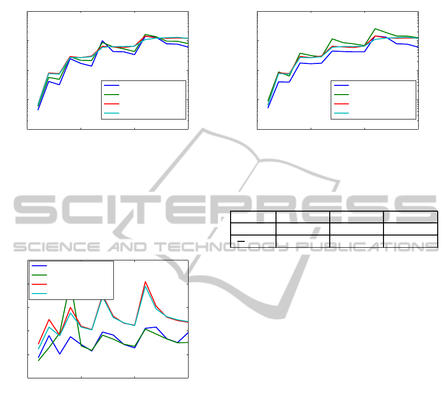
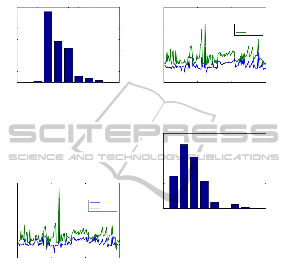
Fig. 1 presents the normalized residuals for the
random examples solved using Newton solver with
line search, and
care
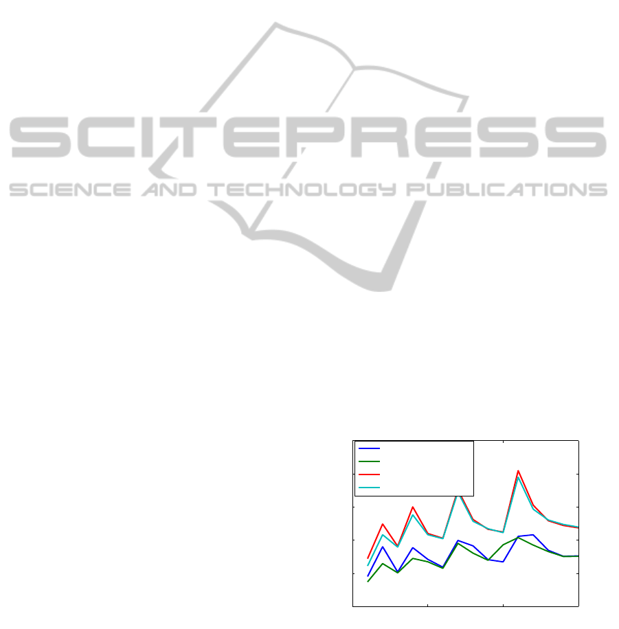
. Fig. 2 presents the CPU times
(computed using the MATLAB pair functions
tic
and
toc
). The y-axis is scaled logarithmically, for
better clarity, since the CPU times vary significantly.
For the largest example, the run time for the Newton
solver and op(M) = M is about half the run time for
care
.
0 5 10 15
10
−12
10
−10
10
−8
10
−6
10
−4
10
−2
Example #
Normalized residuals
Normalized residuals
Newton, op(M) = M
Newton, op(M) = M
T
care, op(M) = M
care, op(M) = M
T
Figure 1: The normalized residuals for random examples
using Newton solver with line search and
care
; n = 200 :
200 : 1000, m = 200 : 200 : n.
Similarly, Fig. 3 and Fig. 4 present the normalized
ICINCO2013-10thInternationalConferenceonInformaticsinControl,AutomationandRobotics
10
0 5 10 15
10
−1
10
0
10
1
10
2
10
3
Example #
CPU time
Elapsed CPU time
Newton, op(M) = M
Newton, op(M) = M
T
care, op(M) = M
care, op(M) = M
T
Figure 2: The CPU times for random examples using New-
ton solver with line search and
care
; n = 200 : 200 : 1000,
m = 200 : 200 : n.
residuals and the CPU times, respectively, when using
standard Newton solver and
care
. The large error for
an example with n = 600, m = 200 (and op(M) =
M
T
) is not typical.
0 5 10 15
10
−12
10
−10
10
−8
10
−6
10
−4
10
−2
Example #
Normalized residuals
Normalized residuals
Newton, op(M) = M
Newton, op(M) = M
T
care, op(M) = M
care, op(M) = M
T
Figure 3: The normalized residuals for random examples
using standard Newton solver and
care
; n = 200 : 200 :
1000, m = 200 : 200 : n.
For both variants, the Newton solver was almost
always faster than
care
. It was also (with one excep-
tion) significantly more accurate. Note that for this set
of tests, the problems with op(M) = M
T
needed more
iterations and CPU time for Newton solver than those
with op(M) = M, especially for the standard Newton
solver. Indeed, the standard Newton solver was most
often over 50% faster than
care
for op(M) = M, but
often over 20% slower than
care
for op(M) = M
T
.
The Euclidean norm of the vectors of normalized
residuals (one normalized residual for each example)
and the mean number of iterations are shown in Ta-
ble 1 for the case op(M) = M.
We have also solved a problem with n = m =
2000, built as above. Newton solver with line search
needed 4 iterations when op(M) = M, and 7 iter-
0 5 10 15
10
−1
10
0
10
1
10
2
10
3
Example #
CPU time
Elapsed CPU time
Newton, op(M) = M
Newton, op(M) = M
T
care, op(M) = M
care, op(M) = M
T
Figure 4: The CPU times for random examples using stan-
dard Newton solver and
care
; n = 200 : 200 : 1000, m =
200 : 200 : n.
Table 1: Normalized residuals 2-norms and mean number
of iterations for random examples.
L. search Standard
care
kr
1:15
k
2
2.98·10
−8
3.01·10
−8
1.55·10
−4
1
15
∑
15
1
k
i
s
5.6 5.33 −
ations when op(M) = M
T
. The CPU times were
about 793 and 1360 seconds, and the normalized
residuals were 8.41·10
−9
and 4.4·10
−9
, respectively.
MATLAB
care
needed about 1350 and 1530 sec-
onds, and the normalized residuals were 2.31 ·10
−7
and 3.66· 10
−7
, respectively. Similarly, when E =
I
n
, the results for the Newton solver were: 4 and
9 iterations, 68 and 469 seconds, and normalized
residuals 1.69· 10
−10
and 3.22 · 10
−13
, respectively.
MATLAB
care
needed 99.4 and 100 seconds, and
the normalized residuals were 1.61 ·10
−11
and 1.01·
10
−11
, respectively.
3.2 Systems from the COMPl
e
ib
Collection
Other tests have been performed for linear systems
from the COMPl
e
ib collection (Leibfritz and Lipin-
ski, 2003; Leibfritz and Lipinski, 2004). This collec-
tion contains 124 standard continuous-time examples
(with E = I
n
), with several variations, giving a total of
168 problems. All but 16 problems (for systems of or-
der larger than 2000, with matrices in sparse format)
have been tried. The performance index matrices Q
and R have been chosen as identity matrices of suit-
able sizes. The matrix L was always zero. Most often
we used the default tolerance.
In a series of tests, we used X
0
set to a zero ma-
trix, if A is stable; otherwise, we tried to initialize the
Newton solver with a matrix computed using the al-
gorithm in (Hammarling, 1982), and when this algo-
ComputationalExperienceinSolvingContinuous-timeAlgebraicRiccatiEquationsusingStandardandModifiedNewton's
Method
11
rithm failed to deliver a stabilizing initialization, we
used the solution provided by the MATLAB function
care
. A zero initialization was used for 44 stable ex-
amples. Stabilization algorithm was tried on 107 un-
stable systems, and succeeded for 91 examples. Fail-
ures occurred for 16 examples. With default toler-
ance, the implementation of the Newton solver used
in the preliminary version of this paper did not im-
prove the
care
solution, returning with 0 iterations.
But, modifying the test at Step 1 of Algorithm N, in
order to continue the calculations at iteration k = 0,
enabled to improve the accuracy of
care
solution for
15 examples. (Only the solution for example ROC5
could not be improved.) The function
care
failed to
solve the Riccati equation for example REA4, with
the error message “There is no finite stabilizing solu-
tion”. This unstable example has been excluded from
our tests, because it could not be stabilized.
We tried both standard and modified Newton’s
method, with or without balancing the coefficient ma-
trices of the Lyapunovequations. The modifiedsolver
needed more iterations than the standard solver for
10 examples only. The cumulative number of itera-
tions with modified and standard solver for all 150
examples was 1654 and 2289, respectively. With bal-
ancing, the total number of iterations was 1657 and
2279, respectively. The mean number of iterations
was about 11, for the modified solver, and 15.2, for
the standard solver. We tried also to use the stabiliza-
tion algorithm whenever possible, including for stable
A matrices. Doing so, the total number of iterations
without balancing was 1796 and 2208, respectively
(1784 and 2207, with balancing).
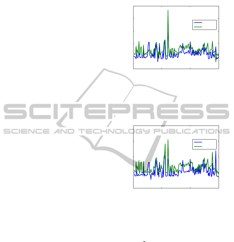
Fig. 5 shows the normalized residuals for the
COMPl
e
ib examples. For clarity, only the results for
Newton solver with line search without balancing and
for
care
are plotted. Note that the normalized resid-
ual is higher than 1 for the TL example when using
care
. (Its value is 2.13·10
3
for
care
, but 1.09·10
−3
for the Newton solver, and 1.32 ·10
−3
, using a stabi-
lizing X
0
6= 0.) The matrices A and B of this example
have norms of order 10
14
and are poorly scaled (the
minimum magnitude in A is of order 10
−4
). Omitting
example TL, the maximum normalized residual was
of order 10
−6
for the standard Newton solver, and of
order 10
−9
(10
−10
with balancing) for the modified
solver and
care
.
Similarly, Fig. 6 shows the relativeresiduals, com-
puted in a similar manner with that used in
care
. The
maximum value of these residuals is 8.98 ·10
−9
for
the modified Newton solver (for example ROC5), and
3.16·10
−5
for
care
(for example TL) . (Its value was
1 for the standard Newton solver and example TL!)
Omitting example TL, the maximum relative residual
0 50 100 150
10
−20
10
−15
10
−10
10
−5
10
0
10
5
Example #
Normalized residuals
Normalized residuals
Newton
care
Figure 5: The normalized residuals for examples from the
COMPleib collection, using Newton solver with line search
without balancing and
care
.
was of order 10
−7
for the standard Newton solver and
of order 10
−6
for
care
.
0 50 100 150
10
−20
10
−15
10
−10
10
−5
10
0
Example #
Relative residuals
Relative residuals
Newton
care
Figure 6: The relative residuals for examples from the
COMPleib collection, using Newton solver with line search
and
care
.
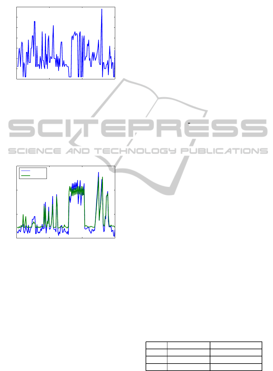
Figure 7 shows the number of iterations of the
Newton solver with line search for the COMPl
e
ib ex-
amples. The largest number, 34, was applied for ex-
ample CM5
IS, with order n = 480, and m = 1.
Similarly, Fig. 8 shows the elapsed CPU times.
Although the modified Newton method was faster
than
care
for 100 examples, out of 150, the sum of
the CPU times was about 64% larger than for
care
.
This is mainly due to the fact that, with the chosen
initialization, some large examples (mainly, 15 exam-
ples in the HF2D class) required at least 19 iterations.
The standard Newton solver was globally over 25%
slower than the solver with line search. The balanc-
ing option increased the CPU times by less than 4%
in both cases. When using stabilizing X
0
6= 0, the
speed-up of the modified Newton solver increased by
about 30%; the main contribution came from solving
the ARE for example CM6 (n = 960, m = 1) in just
ICINCO2013-10thInternationalConferenceonInformaticsinControl,AutomationandRobotics
12
0 50 100 150
0
5
10
15
20
25
30
35
Example #
Number of iterations
Number of iterations (Newton with line search)
Figure 7: The number of iterations performed by the New-
ton solver with line search for examples from the COMPleib
collection.
one iteration, compared to 19 iterations needed when
X
0
= 0 was used. (Note that the stabilization algo-
rithm did not work for example CM6, so X
0
was set
to the
care
solution.) Clearly, a good initialization
could significantly reduce the number of iterations.
0 50 100 150
10
−4
10
−2
10
0
10
2
Example #
CPU time
Elapsed CPU time
Newton
care
Figure 8: The elapsed CPU time needed by the Newton
solver with line search and MATLAB
care
for examples
from the COMPleib collection.
When the solution returned by
care
was used to
initialize the Newton solver variants for all COMPl
e
ib
examples, with default tolerance and without the
modification, mentioned before, of the test at Step 1,
the total number of iterations was 69, namely 50 it-
erations for TL, and one iteration for other 19 ex-
amples. The remaining examples were solved with-
out any iterations, since
care
results were accurate
enough with the default tolerance. The sum of the
CPU times for Newton solver was about 2.4 seconds,
compared to about 53.8 seconds for
care
. The nor-
malized residual decreased to 1.05·10
−3
for exam-
ple TL, but the relative residual slightly increased to
9.76·10
−6
. Omitting the example TL, the maximum
normalized residual decreased to 9.17·10
−10
(for ex-
ample EB6, with n = 160, m = 1), and the maximum
relative residual was 3.85·10
−10
(for example ISS2,
with n = 270, m = 3).
After modifying the test at Step 1 to force the
solver to try at least an update, and after adding a
test of relative residual, the total number of itera-
tions increased to 159, namely 11 iterations for ex-
ample TL, zero iterations for ROC5, and one itera-
tions for the other examples. The sum of the CPU
times for Newton solver was then about 8.3 sec-
onds. The normalized residual for example TL var-
ied in between 9.3 ·10
−4
and 1.3·10
−3
for the four
variants (with/without line search and with/without
balancing), and the relative residual varied between
1.61 ·10
−11
and 2.05·10
−11
. Omitting the example
TL, the maximum normalized residual decreased to
6.9·10
−13
for Newton solver, and 3.6·10
−9
for
care
(for example HF2D IS5, with n = 5, m = 2), and the
maximum relative residual was 8.42·10
−13
(for ex-
ample CBM, with n = 348, m = 1). The decision to
keep this modification of the tests was based on these
improved results.
We used the same initialization provided by
care
with values for the tolerance parameter τ set to 10
−12
,
10
−14
, and relative machine precision, ε
M
.
For τ = 10
−12
, the behavior was identicalwith that
for the default τ. For τ = 10
−14
, example TL needed
50 iterations without convergence (the tolerance be-
ing too small), one example needed 6 iterations, 2 ex-
amples needed 5 iterations, 3 examples needed 4 iter-
ations, 14 examples needed 3 iterations, 9 examples
needed 2 iterations, 119 examples needed one itera-
tion, and ROC5 needed no iteration. The repartition
of the number of iterations for τ = ε
M
is shown in
the bar graph from Fig. 9, where TL example was ex-
cluded, for clarity. Only for ROC5 example, the New-
ton solver returned before finishing the first iteration
(reporting 0 iterations); it found that no improvement
of X
0
is numerically possible, since the norm of the
correction t
0
N
0
, 3.07·10
−14
, was too small compared
to the norm of X
0
, which is 1.41 ·10
4
. (The normal-
ized residual value for X
0
was 4.88 ·10
−18
.) Omit-
ting TL, the maximum normalized residual reduced
to 6.9·10
−13
for τ = 10
−12
, and to about 3.5 ·10
−13
for smaller values of τ. Performance results are sum-
marized in Table 2.
Table 2: Summary of performance results for small toler-
ance τ and initialization by MATLAB
care
.
τ Total iterations Sum of CPU times
10
−12
198 10.83
10
−14
257 23.79
ε
M
344 26.23
ComputationalExperienceinSolvingContinuous-timeAlgebraicRiccatiEquationsusingStandardandModifiedNewton's
Method
13
0 1 2 3 4 5 6
0
10
20
30
40
50
60
70
Repartition of the number of iterations
Number of examples
Number of iterations
Figure 9: Bar graph showing the repartition of the num-
ber of iterations for examples from the COMPleib collec-
tion, using Newton solver with line search without balanc-
ing, initialization using
care
and tolerance relative machine
precision.
Fig. 10 shows the normalized residuals for the New-
ton solver with line search, initialized by
care
, and
with tolerance τ = ε
M
. Clearly, Newton solver re-
duces the residuals by several orders of magnitude,
compared to
care
.
0 50 100 150
10
−20
10
−15
10
−10
10
−5
10
0
10
5
Example #
Normalized residuals
Normalized residuals
Newton
care
Figure 10: The normalized residuals for examples from the
COMPleib collection, using Newton solver with line search
without balancing, initialization using
care
and tolerance
relative machine precision.
Fig. 11 shows similarly the relative residuals. Ex-
cept for ROC5, Newton solver always reduces the
residuals, often by several orders of magnitude, com-
pared to
care
. Fig. 12 shows by a bar graph the size
of this improvement. Specifically, the improvement is
of seven orders of magnitude for one example, six or-
ders for three examples, four ordersfor five examples,
etc. For 114 examples, the improvement is between
one and three (inclusive) orders of magnitude.
0 50 100 150
10
−20
10
−15
10
−10
10
−5
10
0
Example #
Relative residuals
Relative residuals
Newton
care
Figure 11: The relative residuals for examples from the
COMPleib collection, using Newton solver with line search
without balancing, initialization using
care
and tolerance
relative machine precision.
1 2 3 4 5 6 7 8
0
10
20
30
40
50
60
Improvement of relative residuals
Number of examples
i
Figure 12: Bar graph showing the improvement of the rela-
tive residuals for examples from the COMPleib collection,
using Newton solver with line search without balancing, ini-
tialization using
care
and tolerance relative machine preci-
sion. The height of the i-th vertical bar indicates the num-
ber of examples for which the improvement was between
i-1 and i orders of magnitude.
4 CONCLUSIONS
Basic theory and improved algorithms for solving
continuous-time algebraic Riccati equations using
Newton’s method with or without line search have
been presented. Algorithmic details for the devel-
oped solvers, the main computational steps (finding
the Newton direction, finding the Newton step size),
and convergence tests are described. The usefulness
of such solvers is demonstrated by the results of an
extensive performance investigation of their numeri-
cal behavior, in comparison with the results obtained
using the widely-used MATLAB function
care
. Ran-
domly generated systems with orders till 1000 (and
even a system with order 2000),as well as the systems
ICINCO2013-10thInternationalConferenceonInformaticsinControl,AutomationandRobotics
14

from the large COMPl
e
ib collection, are considered.
The numerical results most often show significantly
improved accuracy (measured in terms of normalized
and relative residuals), and greater efficiency. The re-
sults strongly recommend the use of such algorithms,
especially for improving, with little additional com-
puting effort, the solutions computedby other solvers.
ACKNOWLEDGEMENTS
Part of this work was done many years ago in a
research stay at the Technical University Chemnitz,
Germany, during November 1 – December 20, 2005,
with the financial support from the German Science
Foundation. The long cooperation with Peter Benner
from Technical University Chemnitz and Max Planck
Institute for Dynamics of Complex Technical Sys-
tems, Magdeburg, Germany, is much acknowledged.
Thanks are also addressed to Martin Slowik from In-
stitut f¨ur Mathematik, Technical University Berlin,
who worked out (till 2005) a preliminary version of
the SLICOT codes for continuous-timealgebraic Ric-
cati equations. The work has been recently resumed
by the author. Finally, the continuing support from
the NICONET e.V. is warmly acknowledged.
REFERENCES
Abels, J. and Benner, P. (1999). CAREX—A collec-
tion of benchmark examples for continuous-time al-
gebraic Riccati equations (Version 2.0). SLICOT
Working Note 1999-14, Katholieke Universiteit Leu-
ven, ESAT/SISTA, Leuven, Belgium. Available from
http://www.slicot.org.
Anderson, B. D. O. and Moore, J. B. (1971). Linear
Optimal Control. Prentice-Hall, Englewood Cliffs,
New Jersey.
Anderson, E., Bai, Z., Bischof, C., Blackford, S., Demmel,
J., Dongarra, J., Du Croz, J., Greenbaum, A., Ham-
marling, S., McKenney, A., and Sorensen, D. (1999).
LAPACK Users’ Guide: Third Edition. Software ·En-
vironments · Tools. SIAM, Philadelphia.
Arnold, III, W. F. and Laub, A. J. (1984). Generalized
eigenproblem algorithms and software for algebraic
Riccati equations. Proc. IEEE, 72(12):1746–1754.
Benner, P. (1997). Contributions to the Numerical So-
lution of Algebraic Riccati Equations and Related
Eigenvalue Problems. Dissertation, Fakult¨at f¨ur Math-
ematik, Technische Universit¨at Chemnitz–Zwickau,
D–09107 Chemnitz, Germany.
Benner, P. (1998). Accelerating Newton’s method for
discrete-time algebraic Riccati equations. In Beghi,
A., Finesso, L., and Picci, G., editors, Mathemati-
cal Theory of Networks and Systems, Proceedings of
the MTNS-98 Symposium held in Padova, Italy, July,
1998, pages 569–572. Il Poligrafo, Padova, Italy.
Benner, P. and Byers, R. (1998). An exact line search
method for solving generalized continuous-time alge-
braic Riccati equations. IEEE Trans. Automat. Contr.,
43(1):101–107.
Benner, P., Byers, R., Losse, P., Mehrmann, V., and
Xu, H. (2007). Numerical solution of real skew-
Hamiltonian/Hamiltonian eigenproblems. Technical
report, Technische Universit¨at Chemnitz, Chemnitz.
Benner, P., Byers, R., Mehrmann, V., and Xu, H. (2002).
Numerical computation of deflating subspaces of
skew Hamiltonian/Hamiltonian pencils. SIAM J. Ma-
trix Anal. Appl., 24(1):165–190.
Benner, P., Kressner, D., Sima, V., and Varga, A.
(2010). Die SLICOT-Toolboxen f¨ur Matlab. at—
Automatisierungstechnik, 58(1):15–25.
Benner, P., Mehrmann, V., Sima, V., Van Huffel, S., and
Varga, A. (1999). SLICOT — A subroutine library
in systems and control theory. In Datta, B. N., ed-
itor, Applied and Computational Control, Signals,
and Circuits, volume 1, chapter 10, pages 499–539.
Birkh¨auser, Boston.
Benner, P. and Sima, V. (2003). Solving algebraic Riccati
equations with SLICOT. In CD-ROM Proceedings
of The 11th Mediterranean Conference on Control
and Automation MED’03, June 18–20 2003, Rhodes,
Greece. Invited session IV01, “Computational Tool-
boxes in Control Design”, Paper IV01-01, 6 pages.
Byers, R. (1987). Solving the algebraic Riccati equa-
tion with the matrix sign function. Lin. Alg. Appl.,
85(1):267–279.
Ciubotaru, B. and Staroswiecki, M. (2009). Comparative
study of matrix Riccati equation solvers for paramet-
ric faults accommodation. In Proceedings of the 10th
European Control Conference, Budapest, Hungary,
pages 1371–1376.
Francis, B. A. (1987). A Course in H
∞
Control Theory,
volume 88 of Lect. Notes in Control and Information
Sciences. Springer-Verlag, New York.
Gardiner, J. D. and Laub, A. J. (1986). A generalization of
the matrix sign function solution for algebraic Riccati
equations. Int. J. Control, 44:823–832.
Hammarling, S. J. (1982). Newton’s method for solving the
algebraic Riccati equation. NPC Report DIIC 12/82,
National Physics Laboratory, Teddington, Middlesex
TW11 OLW, U.K.
J´onsson, G. F. and Vavasis, S. (2004). Solving polynomials
with small leading coefficients. SIAM J. Matrix Anal.
Appl., 26(2):400–414.
Kleinman, D. L. (1968). On an iterative technique for Ric-
cati equation computations. IEEE Trans. Automat.
Contr., AC–13:114–115.
Lancaster, P. and Rodman, L. (1995). The Algebraic Riccati
Equation. Oxford University Press, Oxford.
Lanzon, A., Feng, Y., Anderson, B. D. O., and Rotkowitz,
M. (2008). Computing the positive stabilizing solu-
tion to algebraic Riccati equations with an indefinite
quadratic term via a recursive method. IEEE Trans.
Automat. Contr., AC–50(10):2280–2291.
ComputationalExperienceinSolvingContinuous-timeAlgebraicRiccatiEquationsusingStandardandModifiedNewton's
Method
15

Laub, A. J. (1979). A Schur method for solving algebraic
Riccati equations. IEEE Trans. Automat. Contr., AC–
24(6):913–921.
Leibfritz, F. and Lipinski, W. (2003). Description of the
benchmark examples in COMPl
e
ib. Technical report,
Department of Mathematics, University of Trier, D–
54286 Trier, Germany.
Leibfritz, F. and Lipinski, W. (2004). COMPl
e
ib 1.0 – User
manual and quick reference. Technical report, Depart-
ment of Mathematics, University of Trier, D–54286
Trier, Germany.
MATLAB (2011). Control System Toolbox User’s Guide.
Version 9.
Mehrmann, V. (1991). The Autonomous Linear Quadratic
Control Problem. Theory and Numerical Solution,
volume 163 of Lect. Notes in Control and Infor-
mation Sciences (M. Thoma and A. Wyner, eds.).
Springer-Verlag, Berlin.
Mehrmann, V. and Tan, E. (1988). Defect correction meth-
ods for the solution of algebraic Riccati equations.
IEEE Trans. Automat. Contr., AC–33(7):695–698.
Penzl, T. (1998). Numerical solution of generalized Lya-
punov equations. Advances in Comp. Math., 8:33–48.
Penzl, T. (2000). LYAPACK Users Guide. Technical Report
SFB393/00–33, Technische Universit¨at Chemnitz,
Sonderforschungsbereich 393, “Numerische Simula-
tion auf massiv parallelen Rechnern”, Chemnitz.
Raines, III, A. C. and Watkins, D. S. (1992). A class of
Hamiltonian-symplectic methods for solving the alge-
braic Riccati equation. Technical report, Washington
State University, Pullman, WA.
Roberts, J. (1980). Linear model reduction and solution of
the algebraic Riccati equation by the use of the sign
function. Int. J. Control, 32:667–687.
Sima, V. (1981). An efficient Schur method to solve the sta-
bilizing problem. IEEE Trans. Automat. Contr., AC–
26(3):724–725.
Sima, V. (1996). Algorithms for Linear-Quadratic Opti-
mization, volume 200 of Pure and Applied Mathemat-
ics: A Series of Monographs and Textbooks. Marcel
Dekker, Inc., New York.
Sima, V. (2005). Computational experience in solving
algebraic Riccati equations. In Proceedings of the
44th IEEE Conference on Decision and Control and
European Control Conference ECC’ 05, 12–15 De-
cember 2005, Seville, Spain, pages 7982–7987. Om-
nipress.
Sima, V. (2010). Structure-preserving computation of
stable deflating subspaces. In Kayacan, E., editor,
Proceedings of the 10th IFAC Workshop “Adapta-
tion and Learning in Control and Signal Process-
ing” (ALCOSP 2010), Antalya, Turkey, 26–28 Au-
gust 2010 (CD-ROM), 6 pages. IFAC-PapersOnLine,
Volume 10, Part 1, http://www.ifac-papersonline.net/
Detailed/46793.html.
Sima, V. (2011). Computational experience with structure-
preserving Hamiltonian solvers in optimal control. In
Ferrier, J.-L., Bernard, A., Gusikhin, O., and Madani,
K., editors, Proceedings of the “8th International
Conference on Informatics in Control, Automation
and Robotics” (ICINCO 2011), Noordwijkerhout, The
Netherlands, 28–31 July, 2011 (CD-ROM), volume 1,
pages 91–96. SciTePress—Science and Technology
Publications.
Sima, V. and Benner, P. (2006). A SLICOT imple-
mentation of a modified Newton’s method for alge-
braic Riccati equations. In Proceedings of the 14th
Mediterranean Conference on Control and Automa-
tion MED’06, June 28-30 2006, Ancona, Italy (CD-
ROM). Omnipress. Session FEA2: Control Systems
5, Paper FEA2-3.
Sima, V. and Benner, P. (2008). Experimental evaluation
of new SLICOT solvers for linear matrix equations
based on the matrix sign function. In Proceedings
of 2008 IEEE Multi-conference on Systems and Con-
trol. 9th IEEE International Symposium on Computer-
Aided Control Systems Design (CACSD), Hilton Pala-
cio del Rio Hotel, San Antonio, Texas, U.S.A., Septem-
ber 3–5, 2008, pages 601–606. Omnipress.
Van Dooren, P. (1981). A generalized eigenvalue approach
for solving Riccati equations. SIAM J. Sci. Stat. Com-
put., 2(2):121–135.
Van Huffel, S. and Sima, V. (2002). SLICOT and con-
trol systems numerical software packages. In Pro-
ceedings of the 2002 IEEE International Conference
on Control Applications and IEEE International Sym-
posium on Computer Aided Control System Design,
CCA/CACSD 2002, September 18–20, 2002, Scottish
Exhibition and Conference Centre, Glasgow, Scot-
land, U.K., pages 39–44. Omnipress.
Van Huffel, S., Sima, V., Varga, A., Hammarling, S., and
Delebecque, F. (2004). High-performance numeri-
cal software for control. IEEE Control Syst. Mag.,
24(1):60–76.
Varga, A. (1981b). A Schur method for pole assignment.
IEEE Trans. Automat. Contr., AC–26(2):517–519.
ICINCO2013-10thInternationalConferenceonInformaticsinControl,AutomationandRobotics
16
