
SLAM of View-based Maps using SGD
David Valiente, Arturo Gil, Francisco Amor
´
os and
´
Oscar Reinoso
System Engineering Department, Miguel Hern
´
andez University, 03202, Elche, Spain
Keywords:
Visual SLAM, Omnidirectional Images, SGD.
Abstract:
This work presents a solution for the problem of Simultaneous Localization and Mapping (SLAM) based on a
Stochastic Gradient Descent (SGD) technique and using omnidirectional images. In the field of applications
of mobile robotics, SGD has never been tested with visual information obtained from the environment. This
paper suggests the introduction of a SGD algorithm into a SLAM scheme which exploits the benefits of om-
nidirectional images provided by a single camera. Several improvements have been introduced to the vanilla
SGD in order to adapt it to the case of omnidirectional observations. This new SGD approach reduces the
undesired harmful effects provoked by non-linearities which compromise the convergence of the traditional
filter estimates. Particularly, we rely on an efficient map representation, conformed by a reduced set of image
views. The first contribution is the adaption of the basic SGD algorithm to work with omnidirectional observa-
tions, whose nature is angular, and thus it lacks of scale. Former SGD approaches only process one constraint
independently at each iteration step. Instead, we think of a strategy which employes several constraints simul-
taneously as system inputs, with the purpose of improving the convergence speed when estimating a SLAM
solution. In this context, we present different sets of experiments which have been carried out seeking for
validation of our new approach based on SGD with omnidirectional observations. In addition, we compare
our approach with a basic SGD in order to prove the expected benefits in terms of efficiency.
1 INTRODUCTION
The problem of SLAM is an essential aspect in the
field of mobile robots, since a representation of the
environment is necessary for navigation purposes.
The aim of building a map entails a complex process,
since the robot needs to build the map in an incre-
mental manner, while, simultaneously, calculating its
localization inside it. Achieving a coherent map is
problematic due to the noisy sensor data, which af-
fects the simultaneous estimation of the map and the
path followed by the robot.
Traditionally, SLAM approaches have been differ-
entiated according to the representation of the map,
the basic algorithm to compute a solution and the kind
of sensor to gather information of the environment.
Some examples reveal the extensive use of laser range
sensors to construct maps. In this context, two mod-
els were mostly used to estimate map representations:
2D occupancy grid maps based on raw laser (Stach-
niss et al., 2004), and 2D landmark-based maps fo-
cused on the extraction of features, described from
laser measurements (Montemerlo et al., 2002).
The use of visual information has lately set a new
tendency towards the utilization of cameras. These
sensors outperform former sensors such as laser in
terms of the amount of valid information to build the
map of the environment. Despite the fact that vision
sensors are not as precise as laser sensors, they pro-
vide a huge variety of information of the scene, as
well as they are less expensive, lighter and more ef-
ficient in terms of consumption. In the latter group
there exists several alternatives according to the num-
ber of cameras introduced and their configuration. For
instance, stereo-based approaches (Gil et al., 2010),
in which two calibrated cameras extract relative mea-
surements of a set of 3D visual landmarks, determined
by a visual description. Other approaches present
their estimation of 3D visual landmarks by using a
single camera. In (Civera et al., 2008; Joly and
Rives, 2010) an inverse depth parametrization is car-
ried out to initialize the coordinates of each 3D land-
mark since the distance to the visual landmark can-
not be directly extracted with a single camera. Some
other approaches (Jae-Hean and Myung Jin, 2003)
have also combined two omnidirectional cameras to
exploit the benefits of a wider field, as in the case of a
stereo-pair sensor.
Besides the sensor and the representation of the
map, the kind of algorithm is the main basis to ob-
329
Valiente D., Gil Aparicio A., Amorós Espí F. and Reinoso O..
SLAM of View-based Maps using SGD.
DOI: 10.5220/0004482603290336
In Proceedings of the 10th International Conference on Informatics in Control, Automation and Robotics (ICINCO-2013), pages 329-336
ISBN: 978-989-8565-71-6
Copyright
c
2013 SCITEPRESS (Science and Technology Publications, Lda.)

tain a solution for the problem of SLAM. In this
sense, different SLAM algorithms have been ex-
tensively used, differentiating between online meth-
ods such as, EKF (Davison and Murray, 2002),
Rao-Blackwellized particle filters (Montemerlo et al.,
2002) and offline algorithms, such as, for example,
Stochastic Gradient Descent (Grisetti et al., 2007).
Thus, the success of an efficient SLAM solution is
closely dependent on the suitability of the combi-
nation between data sensor information, map repre-
sentation model and the SLAM algorithm. A large
amount of research has been conducted to obtain the
map representation, dealing simultaneously with the
estimation of the position of a set of 3D visual land-
marks expressed in a general reference system (Davi-
son and Murray, 2002; Gil et al., 2010; Andrew
J. Davison et al., 2004; Civera et al., 2008). They
rely on the capability of an EKF filter to converge to
a proper solution for the problem of SLAM. More re-
cently (Valiente et al., 2012), also based on EKF, pro-
posed a different representation of the environment,
where the map is formed by the position and orienta-
tion of a reduced set of image views in the environ-
ment. The most distinctive novelty of this representa-
tion is the capability to compute a relative movement
between views, which allows to retrieve the local-
ization of the robot and simultaneously it provides a
compact representation of the environment by means
of a reduced set of views. Such technique establishes
an estimation of a state vector which includes the
map and the current localization of the robot at each
timestep k. The estimation of the transition between
states at k and k + 1 takes into account the wheel’s
odometry as initial estimate, and the observation mea-
surements gathered by sensors. The major problem-
atic experienced by these methods based on an EKF
is the difficulty to keep the convergence of the estima-
tion when gaussian errors appear in the observation,
since they usually cause important data association
problems (Neira and Tard
´
os, 2001). A visual obser-
vation as omnidirectional is susceptible to introduce
non-linearties and therefore responsible for those er-
rors.
Some approaches have demonstrated considerable
improvements thanks to the assumption of a novel
representation of the map (Valiente et al., 2012), com-
posed by a subset of omnidirectional images, denoted
as views. Each view is representative of a large area
of the map since it may encapsulate a huge amount of
visual information in its neighborhood. Considering
a reduced set of images, it leads to a simplification
of the map representation. The scheme allows for a
simple-computation of an observation measurement:
given two images acquired at two poses of the robot,
a specific subset of significant points between images
can be processed in order to get a motion transforma-
tion which establishes the movement between the two
poses of the robot. This approach mitigates the main
EKF’s efficiency issue related to the high number of
variables needed to estimate a solution at each itera-
tion. Here, the number of landmarks, seen as views, is
drastically reduced and thus the time consumption for
the state’s re-estimation too. On the other hand, the
problematic of convergence associated to EKF’s al-
gorithms still exists. In this work we rely on the SGD
algorithm, which it is known to outperform EKF’s
SLAM results. Our main goal is to benefit from
our visual observation model adapted to this kind of
SLAM solution algorithm based on SGD. Note that
even with SGD, solution’s convergence is not trivial
when the observation does not provide range distance
values. We also propose a variation in the procedure
to estimate the solution. Traditionally, either odom-
etry or observation are independently used in order
to iterate up to reach a final solution. By contrast,
we suggest the use of the information provided by
several observations at the same time to quickly find
the SLAM solution. This proposal gives the first im-
pression of being liable to cause an increase of the
required computational resources. Nevertheless, we
have concentrated on the updating of several stages
of the iterative optimization process aiming at preven-
tion from possible harmful bottleneck effects.
The paper is divided as follows: Section 2 ex-
plains the SLAM problem in the mentioned context.
Then, in Section 3 we detail the specifications of a
Maximum Likelihood algorithm such as SGD. Sec-
tion 4 describes the main novelties provided by this
approach. Next, Section 5 shows the experimental re-
sults to test the suitability of the model and its bene-
fits. Finally, Section 6 is referred to the result’s anal-
ysis in order to extract a general conclusion.
2 SLAM
A visual SLAM technique is expected to retrieve a
feasible estimation of the position of the robot in-
side a certain environment, which it has to be well-
determined by the estimation as well. In our ap-
proach, the map is composed by a set of omnidirec-
tional images obtained from different poses in the en-
vironment, denoted as views. These views do not rep-
resent any physical landmarks, since they will be con-
stituted by an omnidirectional image captured at the
pose x
l
= (x
l
,y
l
,θ
l
) and a set of interest points ex-
tracted from that image. Such arrangement, allows us
to exploit the capability of an omnidirectional image
ICINCO2013-10thInternationalConferenceonInformaticsinControl,AutomationandRobotics
330

to gather a large amount of information in a simple
image, due to its large field of view. Thus, an im-
portant reduction is achieved in terms of number of
variables to estimate the solution.
The pose of the mobile robot at time t will be de-
noted as x
v
= (x
v
,y
v
,θ
v
)
T
. Each view i ∈ [1, . . . , N]
is constituted by its pose x
l
i
= (x
l
,y
l
,θ
l
)
T
i
, its uncer-
tainty P
l
i
and a set of M interest points p
j
expressed
in image coordinates. Each point is associated with a
visual descriptor d
j
, j = 1, . . . , M.
Thus, the augmented state vector is defined as:
¯x =
x
v
x
l
1
x
l
2
··· x
l
N
T
(1)
where x
v
= (x
v
,y
v
,θ
v
)
T
is the pose of the moving ve-
hicle and x
l
N
= (x
l
N
,y
l
N
,θ
l
N
) is the pose of the N-view
that exist in the map.
2.1 Observation Model
According to the view-based representation of the
map, it is also necessary to describe an observation
model. The versatility of using omnidireccional im-
ages makes it possible to extract an observation mea-
surement which defines the motion transformation be-
tween two poses (Valiente et al., 2012), as seen in Fig-
ure 1. Actually, these poses represent the positions
where the robot acquired two specific images. To that
effect, only two images with a set of corresponding
points between them are required to obtain the trans-
formation. Following, the observation measurement
is described:
z
t
=
φ
β
=
arctan(
y
l
N
−y
v
x
l
N
−x
v
) − θ
v
θ
l
N
− θ
v
!
(2)
where the angle φ is the bearing at which the view
N is observed and β is the relative orientation be-
tween the images. The view N is represented by
x
l
N
= (x
l
N
,y
l
N
,θ
l
N
), whereas the pose of the robot
is described as x
v
= (x
v
,y
v
,θ
v
). Both measurements
(φ,β) are represented in Figure 1.
3 MAXIMUM LIKELIHOOD
MAPPING
3.1 Problem Specifications
A graph-oriented map is composed by a set of nodes
defining the poses traversed by the robot and the land-
marks initialized into the map. The state vector s
t
encodes this representation through a set of variables
which are expressed in the following manner:
s
t
=
(x
0
,y
0
,θ
0
),(x
1
,y
1
,θ
1
)... (x
n
,y
n
,θ
n
)
(3)
Figure 1: Motion relation between two poses of the robot
with two omnidirectional images acquired at that poses.
The same motion relation is shown in the images with spe-
cific observation variables φ and β indicated.
being (x
n
,y
n
,θ
n
) the 3D coordinates in a general ref-
erence system. A complementary subset of edges rep-
resents the relationships between nodes, by means of
either distance measurements generated by the odom-
etry or observations measurements provided by the
on board sensors. Both measurements are commonly
known as constraints and denoted as δ
ji
, where j in-
dicates the observed node, seen from node i. The gen-
eral objective stated by these kind of methods (Olson
et al., 2006; Grisetti et al., 2007) is to minimize the
error likelihood expressed as:
P
ji
(s) ∝ ηexp (−
1
2
( f
ji
(s) − δ
ji
)
T
Ω
ji
( f
ji
(s) − δ
ji
))
(4)
being f
ji
(s) a function dependent on the state s
t
and
both nodes j and i. The difference between f
ji
(s) and
δ
ji
expresses the error deviation between nodes. Such
error term is weighted by the information matrix:
Ω
ji
= Σ
−1
ji
(5)
where Σ
−1
ji
is the associated covariance, aimed at in-
troducing the uncertainty of the measurements. The
assumption of logarithmic notation leads to:
F
ji
(s) ∝ ( f
ji
(s) − δ
ji
)
T
Ω
ji
( f
ji
(s) − δ
ji
) (6)
= e
ji
(s)
T
Ω
ji
e
ji
(s) = r
ji
(s)
T
Ω
ji
r
ji
(s) (7)
SLAMofView-basedMapsusingSGD
331

being e
ji
(s) the error determined by f
ji
(s)-δ
ji
(s),
also denoted as r
ji
(s) to emphasize its condition of
residue. Finally, the global problem seeks the min-
imization of the objective function which represents
the accumulated error:
F(s) =
∑
h j,ii∈G
F
ji
(s) =
∑
h j,ii∈G
r
ji
(s)
T
Ω
ji
r
ji
(s) (8)
where G = {h j
1
,i
1
i,h j
2
,i
2
i...} defines the subset of
particular constraint conforming the map, either per-
taining to odometry or observation measurements.
3.2 Problem Solution. SGD
Once the formulation of the problem has been pre-
sented, it has to be detailed the Stochastich Gradi-
ent Descent algorithm. The basic goal is to compute
in an iterative manner a closer estimation to reach
a valid solution for the SLAM problem. The basis
of a SGD method lays on the minimization of (8)
through derivative optimization techniques. The es-
timated state vector is obtained as:
s
t+1
= s
t
+ ∆s (9)
where ∆s expresses a certain update with respect to s
t
,
term which is sequentially generated by means of the
constraint optimization procedure. It is worth noting
that in a general case, this update is calculated inde-
pendently at each step by using only a simple con-
straint, that is to say ∆s
n
= f (δ
ji
). The general ex-
pression for the transition between s
t
and s
t+1
has the
following form:
s
t+1
= s
t
+ λ · H
−1
J
T
ji
Ω
ji
r
ji
(10)
• λ is a learning factor to re-scale the term
H
−1
J
T
ji
Ω
ji
r
ji
. Normally, λ takes decreasing val-
ues following the criteria λ = 1/n, where n is the
iteration step. This strategy pretends to quickly
reach the final solution for higher values of λ. In
case it is close to the optimum, lower values of λ
are expected to prevent from oscillations around
the final solution.
• H is the Hessian matrix, calculated as J
T
ΩJ,
and it represents the shape of the error function
through a preconditioning matrix to scale the vari-
ations of J
ji
. According to (Grisetti et al., 2009),
H can be computed:
H ≈
∑
hi, ji
J
ji
Ω
ji
J
T
ji
(11)
approximating H
−1
to allow a simpler and faster
computation:
H
−1
≈ [diag(H)]
−1
(12)
• J
ji
is the Jacobian of f
ji
with respect to s
t
, J
ji
=
∂ f
ji
∂s
. It converts the error deviation into a spacial
variation.
• Ω
ji
is the information matrix associated to a con-
straint. Ω
ji
= Σ
−1
ji
, being Σ
ji
the covariance matrix
corresponding with the constraint observations δ
ji
This scheme updates the estimation by computing
the rectification introduced by each constraint at each
iteration step respectively. Despite the learning factor
to reduce the weight by which each constraint updates
the estimation, the procedure can lead to an inefficient
method to reach a stable solution, since undesired os-
cillations may occur due to the stochastic nature of
the constraints’ selection. For this reason, we pro-
pose an optimization process which takes into account
several constraints at the same iteration. It might be
thought that same drawbacks of a general case could
arise, in addition of some other inconveniences such
as undesired overloads of time, as a consequence of
the simultaneous processing of several constraints at
the same iteration. However, we have modified some
calculations at specific stages of the algorithm in or-
der to maintain the time requirements and even to re-
duce them. As a results, we achieved improved con-
vergence ratios in terms of speed. Further details will
be provided in the next sections.
4 MODIFIED SGD
The first assumption to consider is the redefined state
vector s
t
, which will be treated as a set of incremental
variables. Pose incremental is defined as:
s
inc
t
=
x
0
y
0
θ
0
dx
1
dy
1
dθ
1
...
dx
n
dy
n
dθ
n
=
x
0
y
0
θ
0
x
1
− x
0
y
1
− y
0
θ
1
− θ
0
x
2
− x
1
y
2
− y
1
θ
2
− θ
1
...
x
n
− x
n−1
y
n
− y
n−1
θ
n
− θ
n−1
(13)
where (dx
i
,dy
i
,dθ
i
) encode the variation between
consecutive poses in coordinates of the global refer-
ence system. A global encoding has the main draw-
back of not being capable to update more than one
node and its adjacents per constraint. Regarding a rel-
ative codification of the sate, it arises the problem of
ICINCO2013-10thInternationalConferenceonInformaticsinControl,AutomationandRobotics
332

non-linearities in J
ji
. By contrast, an incremental state
vector allows a single constraint to generate a varia-
tion on every pose. In this framework, ∆s (9) affects
all poses because the state vector is differentially en-
coded.
It should be noticed that in this approach we are
dealing with a visual observation given by an om-
nidirectional camera. This fact makes us to adapt
the equations defined in the previous section, since
the nature of the constraints are not only metrical
like odometry’s constraints. According to (2), given
two nodes, the observation measurement allows us to
determine a specific motion transformation between
them up to a scale factor. Therefore, the omnidirec-
tional measurements and the incremental represen-
tation require the reformulation of several terms in-
volved in the estimation. Following, we detail all the
terms which needed to be modified and recalculated.
• The first adaption made was in f
ji
, differentiating
between odometry:
f
odo
j,i
(s) =
dx
j
dy
j
dθ
j
+
dx
j−1
dy
j−1
dθ
j−1
+ ··· +
dx
i
dy
i
dθ
i
(14)
where (dx
j
,dy
j
,dθ
j
) are defined in (13), and vi-
sual observation constraints:
f
visual
j,i
(s) =
φ
β
=
arctan(
dy
j
−dy
i
dx
j
−dx
i
) − dθ
i
dθ
j
− dθ
i
!
(15)
where φ and β are directly computed as the obser-
vation measurement (Valiente et al., 2012) which
expresses the relation between the omnidirec-
tional images and the pose codification (13). In-
spection of Figure 1 leads to define (2) and simi-
larly (15).
• Second step, according to this reformulation, is to
recalculate J
ji
=
∂ f
ji
∂s
. Please note the importance
of considering the indexes of the corresponding
nodes, either j > i or j < i since the derivatives
vary its form considerably. Furthermore, as seen
above, the dimensions of f
j,i
are different, fact
which has to be taken into account to resize the
rest of the terms involved in the SGD algorithm.
J
j,i
=
∂ f
j,i
∂s
=
∂ f
j,i
(s)
∂s
=
h
∂ f
j,i
(φ)
∂s
,
∂ f
j,i
(β)
∂s
i
(16)
• Thirdly, in this work we suggest the estimation
of the new state s
t+1
by considering several con-
straints at the same time. With this assumption,
we seek for more relevance of constraints’ weight
when searching for the optimal minimum estima-
tion. It is clear that computing more than one
constraint at each algorithm step leads to a cer-
tain overload. By contrast, with this approach, we
reduce the expensive estimation of H. In a gen-
eral case H is computed whenever a single con-
straint is introduced, that is to say, H is computed
as many times as constraints exist. In our case
we only compute H once for each subset of con-
straints introduced simultaneously into the sys-
tem. Consequently we obtain H in a more effi-
cient manner, and therefore we compensate possi-
ble time overloads associated.
5 RESULTS
We have carried out three different experimental sets.
First, in Section 5.1 we show SLAM results obtained
in a simulated scenario to confirm the validity of the
new SLAM approach supported by SGD. Then, Sec-
tion 5.2 presents a comparison of SLAM results us-
ing our approach and a basic SGD algorithm, respec-
tively. Finally, in Section 5.3 we present SLAM re-
sults in an office-like environment.
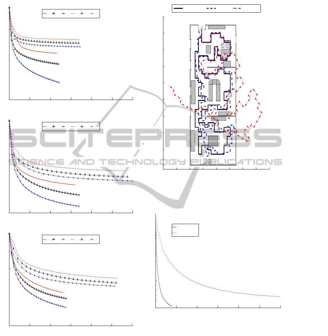
5.1 Experimental Set 1
Assuring the convergence of an SLAM algorithm is of
paramount importance when a new solver technique
is introduced, such SGD. Moreover, the performance
of the new method has to consider certain modifica-
tions to treat with a visual observation model, which
usually adds non-linearities. Figure 2(a) presents a
random simulation environment of 20x20m, where
the robot traverses 300m approximately. The real
path followed by the robot is shown with continuous
line, the odometry is represented with dash-dot line,
whereas the estimated solution is shown with dash
line. A set of views have been placed randomly along
the trajectory. The arrangement of these views is con-
trolled by an appearance ratio between images, so as
to assure a realistic placement of each view. A grid of
circles represents the possible poses where the robot
might move to and gather a new view. The number of
iterations of the SGD algorithm is 25. As it can be ob-
served in Figure 2(a), starting from a noisy first odom-
etry estimate, the final estimation has been rectified
following the tendency of the real path. Figure 2(b)
shows the decreasing evolution of the accumulated er-
ror probability P
ji
(s) in (4), expressed in logarithmic
terms (8), versus the number of iterations. It can be
confirmed the reliability of this new approach to work
SLAMofView-basedMapsusingSGD
333
−10 −5 0 5 10 15 20
−5
0
5
10
15
20
25
X(m)
Y(m)
Solution
Odometry
Ground truth
(a)
0 5 10 15 20 25 30
0
2500
5000
Iteration Step
F(s)
(b)
Figure 2: Figure 2(a) presents a map obtained with the proposed approach in an environment of 20x20m. Continuous line
shows the ground truth, dash-dot line the odometry and dash line the estimated solution. Figure 2(b) shows the accumulated
error probability F(s) along the number of iterations.
with omnidirecctional observations since it provides
a correct solution.
5.2 Comparing Experiments
The following experiments has been conducted to
compare our approach with a basic SGD in terms of
efficiency. We suggest a strategy to introduce simul-
taneously several constraints into the SGD algorithm.
The main goal is to improve the speed by which the
method iteratively optimizes up to reach a final solu-
tion. In this sense, we have performed a SLAM exper-
iment, where the robot traverses 50m through a given
environment. Again, the number of views in the map
has been randomly placed by following the same pol-
icy explained above. The same experiment has been
repeated 200 times by using the same series of odom-
etry inputs, so as to provide mean values which ex-
press consistent results. Both approaches, ours and
the basic SGD algorithm’s have been compared. We
have modified the number of views N that the robot
is able to observe from each pose. The observation
range r of the robot has also been varied. Figure 3
presents results for the accumulated error probability
F(s), being the objective function which the SGD al-
gorithm seeks to minimize. We compare the solution
obtained with our approach, drawn with continuous
line, versus the solution obtained with a basic SGD
algorithm, drawn with dashed line. Figures 3(a), 3(b)
and 3(c) represent F(s) when the robot observes N=2,
N=4 and N=8 views, respectively. Since we look for a
fair comparison, the x-axis, originally representing it-
eration steps, has been transformed to a normalized
time variable to generate a trustworthy comparison
between both schemes. In terms of efficiency, it may
be proved that the solution provided by our method
outperforms the solution given by a basic SGD, since
the decreasing slope of F(s) is clearly steeper, there-
fore a quicker convergence speed is demonstrated.
This is the main consequence of combining several
constraints at each iteration step, instead of using only
one like a basic SGD used to. It is also remarkable
the relevance of the observation range of the vehicle
r. As seen in Figures 3(a), 3(b) and 3(c), long val-
ues of r provide a better convergence to the detriment
of shorter r. Since the omnidirectional observation is
angular, and it lacks of scale, views seen by the robot
at long distances in the map permit to compute a more
feasible localization.
5.3 Experimental Set 2
The purpose of this experiment is to deal with a more
realistic situation, defined through an office-like en-
vironment. Typical obstructor elements like walls or
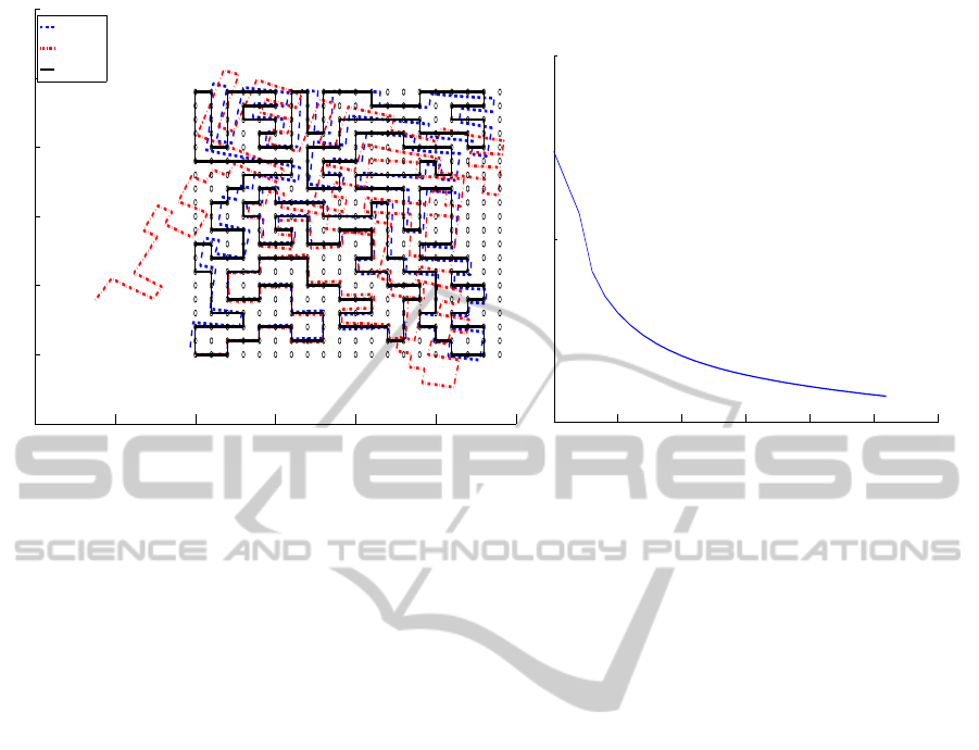
doors have been introduced. Figure 4 describes an en-
vironment of 20x40m which the robot moves through.
The continuous line represents the real path followed
by the robot, the dash-dot line shows the odometry,
whereas the estimated solution with our approach is
ICINCO2013-10thInternationalConferenceonInformaticsinControl,AutomationandRobotics
334
0 1 2 3 4 5 6
1000
2000
3000
4000
Normalized time
F(s)
r
min
r
inter
r
max
r
min
r
inter
r
max
(a)
0 1 2 3 4 5 6
1000
2000
3000
4000
Normalized time
F(s)
r
min
r
inter
r
max
r
min
r
inter
r
max
(b)
0 2 4 6 8 10 12
1000
2000
3000
4000
Normalized time
F(s)
r
min
r
inter
r
max
r
min
r
inter
r
max
(c)
Figure 3: Accumulated error probability F(s) versus time
in a SLAM experiment. Continuous lines show results pro-
vided by the proposed solution whereas the dash lines show
results provided by a basic SGD solution. Figures 3(a), 3(b)
and 3(c) show the results when the number of views ob-
served by the robot is N = 2, N = 4 and N = 8 respectively.
Different length observation ranges r
min
, r
iter
and r
max
are
defined.
−10 −5 0 5 10 15 20 25 30
0
5
10
15
20
25
30
35
40
45
X(m)
Y(m)
Ground truth Solution Odometry
Figure 4: SLAM results in an office-like environment of
20x40m. Continuous line shows the ground truth, dash-dot
line the odometry and dash line the estimated solution.
0 2 4 6 8 10 12
10
3
Normalized time
F(s)
Proposed solution
Basic SGD solution
Figure 5: Comparison of the accumulated error probability
F(s). Continuous line and dash line show F(s) provided by
the proposed approach and a basic SGD algorithm, respec-
tively.
described by a dash line. It may be noticed that in
only 15 iterations of the algorithm the robot is able
to estimate a quiet reliable solution, whose topology
follows the real path’s. On the other hand, the error of
the odometry grows out of bounds. Figure 5 shows a
comparison of the evolution of the accumulated error
SLAMofView-basedMapsusingSGD
335

F(s) versus the time. Once again, it is revealed the
improved capability of our approach to quickly reach
a solution, thus involving a better efficiency. In this
particular case, it can be observed that our approach
requires approximately less than 6 times the compu-
tational needs of a basic SGD to reach an optimum
value.
6 CONCLUSIONS
This work has presented an approach to the SLAM
problem by introducing a SGD algorithm adapted to
work with visual observations. The adoption of SGD
has been intended to overcome instabilities and harm-
ful effects which compromise the convergence of tra-
ditional SLAM algorithms such as filters like EKF.
These problems are mainly caused by a visual obser-
vation, whose nature is non-linear, especially distinc-
tive in omnidirectional observations. We rely on a vi-
sual SLAM approach which builds a map by using
a reduced set of omnidirectional image views. The
retrieval of the pose of the robot is provided by a
single-computation of two views, which directly pro-
vides a motion transformation to relate two poses of
the robot. A basic SGD algorithm has been modi-
fied to work with such unscaled observation model.
In addition, a new strategy has been defined to uti-
lize several constraints simultaneously into the same
SGD iteration, instead of utilizing only one per itera-
tion as former SGD does. We have shown SLAM re-
sults that prove the validity of this new approach with
omnidirectional observations. Moreover, we have es-
tablished a comparison between the results obtained
with our approach and those obtained with a basic
SGD algorithm. Consequently, the suitability of the
approach and its performance has been demonstrated,
but also its benefits in the sense of efficiency.
REFERENCES
Andrew J. Davison, A. J., Gonzalez Cid, Y., and Kita, N.
(2004). Improving data association in vision-based
SLAM. In Proc. of IFAC/EURON, Lisboa, Portugal.
Civera, J., Davison, A. J., and Mart
´
ınez Montiel, J. M.
(2008). Inverse depth parametrization for monocular
slam. IEEE Trans. on Robotics.
Davison, A. J. and Murray, D. W. (2002). Simultaneous lo-
calisation and map-building using active vision. IEEE
Trans. on PAMI.
Gil, A., Reinoso, O., Ballesta, M., Juli
´
a, M., and Pay
´
a, L.
(2010). Estimation of visual maps with a robot net-
work equipped with vision sensors. Sensors.
Grisetti, G., Stachniss, C., and Burgard, W. (2009). Non-
linear constraint network optimization for efficient
map learning. IEEE Trans. on Intelligent Transporta-
tion Systems.
Grisetti, G., Stachniss, C., Grzonka, S., and Burgard, W.
(2007). A tree parameterization for efficiently com-
puting maximum likelihood maps using gradient de-
scent. In Proc. of RSS, Atlanta, USA.
Jae-Hean, K. and Myung Jin, C. (2003). Slam with omni-
directional stereo vision sensor. In Proc. of the IROS,
Las Vegas, USA.
Joly, C. and Rives, P. (2010). Bearing-only SAM using a
minimal inverse depth parametrization. In Proc. of
ICINCO, Funchal, Madeira, Portugal.
Montemerlo, M., Thrun, S., Koller, D., and Wegbreit, B.
(2002). FastSLAM: a factored solution to the simul-
taneous localization and mapping problem. In Proc. of
the 18th national conference on Artificial Intelligence,
Edmonton, Canada.
Neira, J. and Tard
´
os, J. D. (2001). Data association in
stochastic mapping using the joint compatibility test.
IEEE Trans. on Robotics and Automation.
Olson, D., Leonard, J., and Teller, S. (2006). Fast itera-
tive optimization of pose graphs with poor initial esti-
mates. In Proc of ICRA, Orlando, USA.
Stachniss, C., Grisetti, G., Haehnel, D., and Burgard, W.
(2004). Improved Rao-Blackwellized mapping by
adaptive sampling and active loop-closure. In Proc.
of the SOAVE, Ilmenau, Germany.
Valiente, D., Gil, A., Fern
´
andez, L., and Reinoso, O. (2012).
View-based maps using omnidirectional images. In
Proc. of ICINCO, Rome, Italy.
ICINCO2013-10thInternationalConferenceonInformaticsinControl,AutomationandRobotics
336
