Mimicking Complexity

Automatic Generation of Models for the Development of Self-adaptive Systems

emy Boes, Pierre Glize and Fr

eric Migeon

Institut de Recherche en Informatique de Toulouse, Universit

e Paul Sabatier, Toulouse, France

Keywords:

Complex Systems Modeling, Multi-Agent Systems, Self-tuning, Self-composition.

Abstract:

Many methods for complex systems control use a black box approach where the internal states and mecha-

nisms of the controlled process are not needed to be known. Usually, such systems are tested on simulations

before their validation on the real world process they were made for. These simulations are based on sharp

analytical models of the target process that can be very difﬁcult to obtain. But is it useful in the case of black

box methods? Since the control system only sees inputs and outputs and is able to learn, we only need to

mimic the typical features of the process (such as non-linearity, interdependencies, etc) in an abstract way.

This paper aims to show how a simple and versatile simulator can help the design of systems that have to deal

with complexity. We present a generator of models used in the simulator and discuss the results obtained in

the case of the design of a control system for heat engines.

1 INTRODUCTION

More and more artiﬁcial systems have to deal with

real-world complex processes, like heat engines, bio-

processes or energy management. The design of such

systems usually requires the use of the relevant cor-

responding models so they can be tested on simula-

tions. Unfortunately, models for simulators are very

time consuming to design by the domain experts. This

is due to the great amount of parameters, their interde-

pendencies, the dynamics and the non linearities be-

tween their parts.

Relating our experience in the case of the design

of a heat engine controller, this paper aims to show

that the use of an accurate model is not always re-

quired to ensure the efﬁciency of a system before its

deployment in the real world. Indeed when the sys-

tem is able to learn during its lifetime and to adapt it-

self to the process, the tests concern the learning skills

and the adaptiveness, for which the simulation ﬁdelity

to the domain is not crucial. Following this idea, we

designed simple and versatile abstract black-boxes to

test our system during its development phase. They

do not represent a speciﬁc real-world process, but

only replicate the important features from the adap-

tiveness point of view (such as non-linearity, interde-

pendencies, oscillations or latency). A generator has

been developped to easily build these black-boxes in

order to be able to perform every needed test.

Section 2 gives a short state of the art and explain

why such black-boxes can be adequate, then section 3

details the method to generate them. Section 4 relates

how we use the generated black-boxes and evaluates

their efﬁciency. Finally, we conclude in section 5 with

an analysis of our approach and future improvements.

2 CONTEXT

Our work on complex systems modeling was driven

by our needs in a research project on complex systems

control. This section gives a succinct state of the art

of this ﬁeld before speaking about complex system

modeling and simulation.

2.1 Complex Systems Control

Controlling systems is a generic problem that can be

expressed as ﬁnding which modiﬁcations must be ap-

plied on the inputs in order to obtain the desired ef-

fects on the ouputs. The next paragraphs describe the

main approaches and challenges.

PID - Proportional-Integral-Derivative (PID) are

widely used in the industry. They base the control

on three terms related to the error between the cur-

rent state and the desired state of the process (As-

trom and Hagglund, 1995). PID controllers need a

353

Boes J., Glize P. and Migeon F..

Mimicking Complexity - Automatic Generation of Models for the Development of Self-adaptive Systems.

DOI: 10.5220/0004483003530360

In Proceedings of the 3rd International Conference on Simulation and Modeling Methodologies, Technologies and Applications (SIMULTECH-2013),

pages 353-360

ISBN: 978-989-8565-69-3

 2013 SCITEPRESS (Science and Technology Publications, Lda.)

heavy parametrization work to ﬁt the controlled sys-

tem. Moreover they are not efﬁcient with non-linear

systems and are difﬁcult to deploy to handle more

than one input, which is a severe drawback for com-

plex systems control.

Adaptive Control - To deal with several inputs and

non-linearity, model-based approaches like Model

Predictive Control (MPC) (Nikolaou, 2001) use mod-

els to forecast the behavior of the process in order to

ﬁnd the optimal control scheme. These approaches

are limited by the models they use. Building the mod-

els and ﬁnding the parameters that ﬁt the actual con-

trolled system is an open problem. This will be de-

tailed in 2.2.

Intelligent Control - Intelligent control regroups ap-

proaches that use Artiﬁcial Intelligence methods to

enhance existing controllers and possibly avoid the

use of models. Among these methods we ﬁnd fuzzy

logic (Lee, 1990), expert systems (Stengel, 1991),

neural networks (Hagan et al., 2002), bayesian con-

trollers (Colosimo and Del Castillo, 2007) and multi-

agent systems (Wang, 2001) or (Videau et al., 2011).

These methods often use a black-box approach where

only inputs and outputs values (but not internal vari-

ables and mechanisms) of the process are known by

the controller. Hence intelligent controllers mostly

rely on their learning skills to ﬁnd the optimal con-

trol.

The main challenges in complex systems control

are to deal with interdependencies, non-linearity and

high dynamics. But they also include latency and

noise on the data.

2.2 Complex Systems Modeling

In the context of complex systems control, models can

be used in two ways. Either they are incorporated in

the controller to forecast the process behavior, or they

are used in simulators to test the controller before its

use on the real system.

For instance, many models of engines have been

proposed, such as (Borman, 1964) or the Turbo-

charged Diesel Engine (TDE) model (Jankovic and

Kolmanovsky, 2000). The TDE model has seven pa-

rameters. Using this model in a controller involves

to set them so the model ﬁts the controlled engine.

This is a very difﬁcult task, therefore control meth-

ods like NCGPC (Nonlinear Continuous-time Gen-

eralized Predictive Control) use a simpliﬁed version

with only three parameters (Dabo et al., 2008). How-

ever, ﬁnding the proper values of these parameters re-

mains time consuming and they might become inac-

curate when the engine wears out. The same simpli-

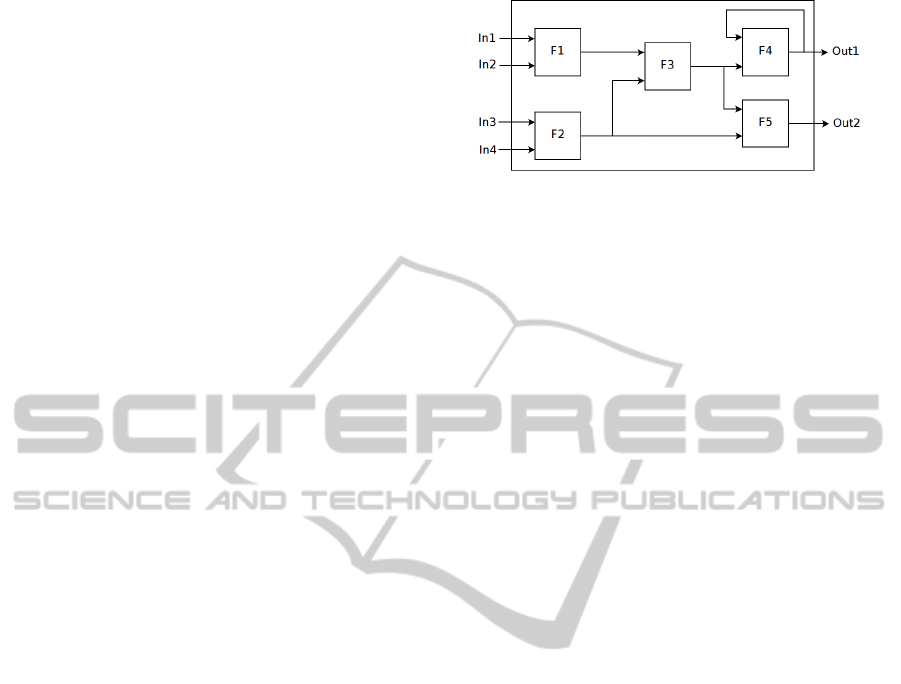
Figure 1: Inside an abstract black-box.

ﬁed TDE model is implemented and used in a simula-

tor to test the NCGPC method, thus avoiding the task

of ﬁnding the parameters values.

Other simulation tools focus on different goals

such as ﬁnding optimal values of engine parame-

ters (Curto-Risso et al., 2009), comparing fuel per-

formances (Zhang et al., 2012) or leading studies on

the behavior of a speciﬁc type of engine (Zhao et al.,

2008). These models are highly speciﬁc and demands

a heavy work of implementation and parametrization.

2.3 Simulation Needs

Our needs in term of simulation come from the devel-

opment of a self-adaptive complex systems controller

meant to be applied on heat engines. We want to be

sure of the system’s adaptation skills before applying

it to real-world engines. Thus, we ﬁrst identiﬁed the

challenging characteristics of engines complexity in

order to simulate them to test our system. In this con-

text, the simulation does not need to be accurate but

only to mimic the complexity of real-world engines.

In other words we want to check the behavior of our

system under various levels of interdependency, vari-

ous numbers of inputs and outputs, with linear or non-

linear outputs, with or without latency (or under any

combination of the previous features), regardless of

the relevance of the data relatively to the real engine.

We also need several instances of each case. None of

the existing heat engine models matches our required

degree of modularity.

Furthermore, existing black-box generation tech-

niques either focus on testing large software with a

discrete state-transitions behavior (Tahat et al., 2001)

or are meant to test software components and not the

whole system (Edwards, 2001). We need to run tests

on the system level with a continuous process.

Hence we use simple yet versatile black-boxes

that mimic the complexity of a real-world process and

that can be automatically generated. The models they

use and their generator are presented in the next sec-

tion.

SIMULTECH2013-3rdInternationalConferenceonSimulationandModelingMethodologies,Technologiesand

Applications

354

Table 1: Input Agents: constraints and behavior.

Constraints Associated Behaviors

Bind Constraint: The agent must bind its output port to

at least one Function Agent. Critical level: 1.

Search for Function Agent with a free input port and bind

to it.

Table 2: Output Agents: constraints and behavior.

Constraints Associated Behaviors

Bind Constraint: The agent must bind its input port to

one (and only one) Function Agent. Critical level: 2.

Search for Function Agent and bind to it.

Path Constraint: The agent must link to every Input

Agents of a speciﬁed list, through a chain of Function

Agents. Output Agents are initialized with a Path con-

straint regarding to the user speciﬁcations. Critical level:

2*size of the list.

Search for a Function Agent linked to some of the tar-

geted Input Agents (if possible), bind to it, and delegate

the Path Constraint.

3 ABSTRACT BLACK-BOXES

In this section we present our abstract black-boxes:

how they are used, what they are made of, and how

they can be easily generated thanks to a multi-agent

system.

3.1 Utilization and Description

Abstract black-boxes are used to simulate a real-

world process in order to test the learning abilities of

an artiﬁcial system during its development. They al-

low to focus on a speciﬁc feature (or on a combination

of them) of complexity, and to make available a large

collection of different instances of the same feature.

They are composed of inputs, outputs and math-

ematical functions. Only inputs and outputs are ob-

servable from the outside. Each of the inputs are

linked to at least one output through a chain of one or

more functions, and vice versa. The chains of func-

tions can be intermingled and can presents cycles.

The role of inputs and outputs is obvious, they are

the link between the functions and the environment of

the black-box. At each timestep, inputs get a value

from the environment and forward it to their linked

functions, functions compute a value and forward it

to their linked neighbors (either other functions, it-

self or outputs), and outputs get the calculated value

of their linked function and forward it to the environ-

ment. To ease the automated generation presented in

3.2, it has been decided to limit the functions to two

arguments and one calculated value. Figure 1 shows

an example of a 4 inputs - 2 outputs generated black-

box, composed of ﬁve functions, containing one cycle

and where each of the four inputs impacts both of the

outputs.

3.2 Generation

A Multi-Agent System, based on the Adaptive Multi-

Agent System theory (Georg

e et al., 2011) and called

BACH (Builder of Abstract maCHines), has been

developped to easily and rapidly generate abstract

black-boxes given user-deﬁned constraints. The user

gives the number of inputs, outputs and functions, de-

ﬁnes the variation range of each input and output, and

which input impacts which output. He also sets a loop

factor which determines the percentage of functions

that have to be in a cycle in the generated black box.

Then agents are created for each component of the

abstract black-box (Input Agents, Output Agents and

Function Agents). There are two main steps to the

generation. First, the self-composition is in charge of

the respect of the structural constraints (interdepen-

dencies and cycles). Then the self-tuning of the func-

tions ensures that the outputs stay in their speciﬁed

range. The self-composition and self-tuning phases

are explained in the next two paragraphs.

3.2.1 Self-Composition

BACH is initialized regarding to the user speciﬁca-

tions: Inputs, Outputs and Functions Agents are cre-

ated and each of them is given a set of individual con-

straints. They have to cooperate and form links be-

tween them to solve these constraints. The resulting

organization is forwarded to the second step of the

generation. The next paragraphs describe the agents,

their constraints and how they solve them.

Architecture and Skills - Agents have inputs and/or

output ports. They can bind their output port to other

agents input ports (and the other way around) but in-

put ports can only be bound once while output ports

can be bound as many times as needed. Input Agents

MimickingComplexity-AutomaticGenerationofModelsfortheDevelopmentofSelf-adaptiveSystems

355

Table 3: Function Agents: constraints and behavior.

Constraints Associated Behaviors

Bind Constraint: The agent must bind its output port to

at least one agent and bind each of its input ports to one

agent. Critical level: 5.

First search a partner to bind the output port, then ﬁnd a

partner for each of the input ports. Partners can be Input

Agents, Output Agents, Function Agents or itself.

Path Constraint: The agent must link to every Input

Agents of a speciﬁed list, either by direct binding or

through a chain of other Function Agents. Function

Agents are not initialized with Path Constraints, but they

eventually receive it from the binding partners on the out-

put port. Critical level: 4*size of the list.

If the agent’s input ports are both free and if the size of the

list is less than or equal to 2, then bind the input ports to

the speciﬁed Input Agents. The constraint is then solved.

Else, if the size of the list is greater than two, bind one of

the input port to another Function Agent, split the list in

half and send one of the half to the new partner, keep the

other. If both of the input ports are already bound, split

the list and send a half to each of the partners.

Cycle Constraint: The agent must be in a cycle. Critical

level: 7

Bind the output port to an agent of its input path, or bind

one of its input ports to an agent in its output path, or bind

one of the input port to its own output port.

do not have any input port and can bind their output

port to Function Agents only. Output Agents do not

have any output port and can bind their input port to

Function Agents only. Finally, Functions Agents have

two input ports, one output port and can bind them to

Input Agents, Output Agents or Function Agents (in-

cluding itself).

Constraints - There are three types of constraints with

which agents can be initialized: Bind Constraints rep-

resent the need for an agent to have all of its input and

output ports bound to another agent, Path Constraints

force agents to link to a speciﬁc list of Input Agents (if

needed through a chain of Function Agents), and Cy-

cle Constraints express the need for a Function Agent

to be part of a cycle.

Behavior - Each constraint has a critical level repre-

senting its relative signiﬁcance. Agents try to solve

their most critical constraint ﬁrst. They have a spe-

ciﬁc behavior for each type of constraint, described in

tables 1, 2 and 3.

The choice of a binding partner is based on two

main criteria: its usefulness and its critical level.

First, the agents are sorted between potential and non-

potential partners, whether they can ﬁll the needs of

the selecting agent or not. Then the potential partner

for which the gain in terms of critical level will be

the best is selected. During the self-composition, an

agent may not ﬁnd any potential partner. This hap-

pens when the user did not speciﬁed enough func-

tions regarding to the number of inputs and outputs

and their interdependencies. In other words the user

speciﬁed an overconstrained problem. In this case,

the system must release a constraint: the number of

functions. Hence the lonely agent creates a new Func-

tion Agent and they bind immediately.

3.2.2 Self-tuning

Once the structure of the black-box is set by the self-

composition phase, interdependencies and cycles an-

swer a part of the user requirements. Now the self-

tuning of the functions ensures that outputs stay in

the user-speciﬁed variation ranges.

Function Agents embed a matrix that is a discrete

representation of their function. The ﬁrst row and the

ﬁrst column are the axis (for the arguments) while

other cells contain the value of the function, thus are

called function cells. Table 4 shows an example of a

function f(x,y) where x varies from 1 to 10, y varies

from 0 to 70 and f from 0 to 100. A linear interpo-

lation is perfomed when needed for the computation

of a value. For instance in table 4, f(3.5,60)=4.5. The

self-tuning of the functions is merely the correct ﬁll-

ing of the matrices.

To do so, each Output Agent sends to its bound

Function Agent a message containing its variation

range. The Function Agent randomly puts each bound

in one of the function cells of its matrix and calculates

the other function cells value v using the formula

v = a ∗ d + m (1)

where m is the value of the closest bound, d is the

Manhattan distance to this bound and a is a positive

coefﬁcient if m is the minimum, negative otherwise.

If the computed v is out of bounds, the value of the

closest bound is affected to the cell instead of v. Once

the function cells are ﬁlled, the variation range of the

Output Agent is respected. Then, the Function Agent

sends a message containing this range to every Func-

tion Agent (possibly itself) bound to its output. Every

agent receiving this message will consequently adjust

the corresponding axis in its matrix. Finally, Input

Agents send their variation range to their bound Func-

tion Agents, who adjust their corresponding axis.

SIMULTECH2013-3rdInternationalConferenceonSimulationandModelingMethodologies,Technologiesand

Applications

356

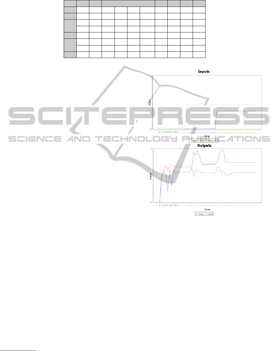
Table 4: A Function Agent’s function matrix: axis (grey) and function cells (white).

− 1 2 3 4 5 6 7 8 9 10

0 37 46 55 64 73 82 73 64 55 46

10 46 55 64 73 82 91 82 73 64 55

20 55 64 73 82 91 100 91 82 73 64

30 50 50 50 50 82 91 82 73 64 55

40 45 36 27 18 50 82 73 64 55 46

50 36 27 18 9 18 50 50 50 50 50

60 27 18 9 0 9 18 27 36 45 54

70 36 27 18 9 18 27 36 45 54 63

3.2.3 Generated Black-boxes

Figure 1 shows the result of the self-composition of

four Input Agents, two Output Agents and ﬁve Func-

tion Agents while table 4 shows the result of the self-

tuning process for a Function Agent. In addition to

the required characteristics of interdependency and

non-linearity, generated black-boxes exhibit oscilla-

tions (periodic or aperiodic), latency and progressive

stabilization, as shown in ﬁgure 2 where inputs are

manually controlled. We can see that the black-box

ﬁrst takes some time to stabilize itself, then a modiﬁ-

cation is applied on input In4. This causes perturba-

tions on outputs Out1 and Out2, then they eventually

stabilize until another modiﬁcation applied on input

In3 causes them to move again.

The next section explains how we used the ab-

stract black-boxes during the development of a heat

engine controller, and compares the results of the tests

on generated black-boxes with those obtained on a

real engine.

4 CASE STUDY: THE DESIGN

OF A CONTROL SYSTEM

FOR HEAT ENGINES

Involved in a national project about heat engine con-

trol named Orianne

, our role was to develop a self-

calibration algorithm for the engine control unit. This

section explains how abstract black-boxes were used

and describes the results obtained both on simulators

and on real engines. In the following paragraphs ES-

CHER is the name of the self-adaptive controller be-

ing developed and tested, and stands for Emergent

Self-adaptive Control for Heat Engine calibRation.

4.1 Method

We deﬁned a two phases process for the development

French acronym for Digital Tool for the Design of En-

gine Control Functions.

Figure 2: Inputs and outputs variations over time of a gen-

erated abstract black-box.

of ESCHER. During the ﬁrst phase, ESCHER was de-

signed and implemented, and all tests were conducted

on abstract black-boxes. Then the second phase con-

sisted in replacing the black-boxes by a real 125cc

gasoline engine. The goal of this second phase is to

validate the use of abstract black-boxes. Indeed, our

software is able to learn the behavior of the generated

black-boxes to ﬁnd the best actions to apply to their

inputs, hence being able to do the same with a real en-

gine would mean that the use of abstract black-boxes

is relevant.

4.2 Results

In this section, more information about ESCHER is

given before results on abstract black-boxes and on a

real engine are shown.

MimickingComplexity-AutomaticGenerationofModelsfortheDevelopmentofSelf-adaptiveSystems

357

4.2.1 ESCHER

ESCHER is a Multi-Agent System based on the Self-

Organizing Controller pattern (Boes et al., 2013).

Its function is to ﬁnd the adequate values of a pro-

cess inputs in order to make the outputs fulﬁlling

user-deﬁned objectives. These objectives are various

(thresholds, optimizations or setpoints), can change

over time and are expressed as criticality functions

that the system tries to lower. ESCHER has no previ-

ous knowledge about the process other than its inputs

and outputs and their variation ranges. It learns in

real-time from the effects of its actions to adjust itself

to the process and ﬁnds the most adequate actions to

apply. In our case, the process is an engine equipped

with its control unit (ECU): the inputs are some of

the parameters of the ECU and the outputs are values

measured on the engine.

In the next paragraphs, we show an example of

test we ran using abstract black-boxes.

4.2.2 Results on Abstract Black-boxes

For this example, we use a black-box with two inputs

(Var0 and Var1) and two outputs (Var2 and Var3). The

objective is to set Var2 and Var3 to the middle of their

range of variation, thus each of the outputs is associ-

ated with a criticality function. ESCHER must ﬁnd

the value of the inputs for which both of the criticality

functions are at their minimum.

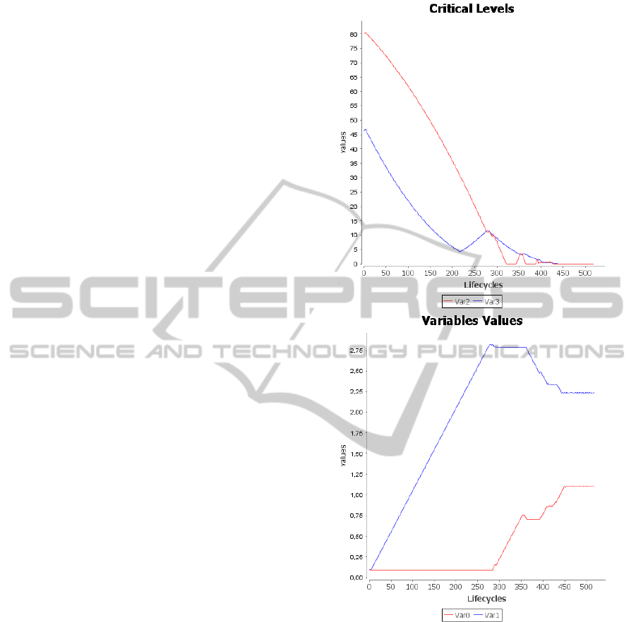
Figure 3 shows the critical levels of the outputs

and the values of the inputs over time. At ﬁrst ES-

CHER increases only Var1. This causes the critical

levels to drop, so ESCHER keeps on this action until

the critical levels begin to increase. Then ESCHER

changes its behavior, modifying its actions (it starts

to increase Var0, lowers and stabilizes Var1, etc) to

maintain the lowering of the critical levels. Finally

both critical levels reach zero, which means the ob-

jectives have been reached. ESCHER now maintains

the black-box in this state.

We have seen that ESCHER is able to ﬁnd the

most adequate values for the inputs of abstract black-

boxes (i.e. for which the critical levels are the lowest).

Now we see in the next paragraph how it behaves with

the real engine.

4.2.3 Results on the Real Engine

The following paragraphs describe an example of the

tests conducted on an engine and validated by do-

main experts. The engine is put in a steady operat-

ing point (deﬁned by its rotational speed and its load).

Then ESCHER has to optimize the engine behavior

by modifying speciﬁc parameters of the ECU.

Figure 3: Test on an abstract black-box: outputs critical

levels (up) and inputs values (bottom).

ESCHER controls the injected fuel mass along

with the ignition advance. Its goal is to maximize the

torque. Figure 4 shows the torque critical level and

both of the controlled parameters. At ﬁrst, ESCHER

decreases both of the controlled parameters, causing

the critical level to rise. It corrects this initial mistake,

increasing the injected fuel mass ﬁrst, then the igni-

tion advance. It eventually ﬁnds the optimum value

for which the critical level is the lowest.

Before analysing these results, it is important to

note that alhough the test shown in 4.2.2 is simple and

easily explainable, BACH was used to generate heav-

ier black boxes that allowed us to enhance ESCHER.

SIMULTECH2013-3rdInternationalConferenceonSimulationandModelingMethodologies,Technologiesand

Applications

358

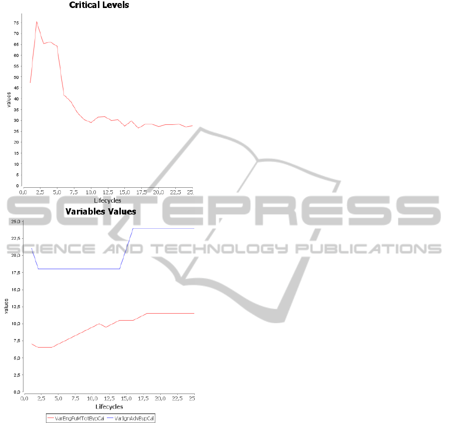
Figure 4: Test on a real engine: torque critical level and

inputs values (injected fuel mass and ignition advance).

4.2.4 Analysis

ESCHER is able to adapt itself and to ﬁnd an op-

timum for abstract black-boxes as well as for the

real engine. This means that the models used in the

black-boxes correctly replicate the main aspects of

the engine in terms of non-linearity and degree of in-

terdependency. The behavior of ESCHER faced to

these main aspects of complexity was properly tested

thanks to the generated abstract black-boxes. How-

ever, some adjustements in the way ESCHER inter-

acts with the process had to be made before obtaining

these results.

This was due to the fact that two important fea-

tures had not been tested with the black-boxes: the

noise on the perceived data, and the latency between

an action and its effects. As ESCHER reacts quickly

to correct its mistakes, the noise did not prevent the

system to work properly, it only made it make a few

more mistakes. But the latency caused more difﬁcul-

ties, the system was not able to ﬁnd the correlation

between its actions and its observations of the pro-

cess behavior. We overcomed this problem by slow-

ing down ESCHER, making it wait three seconds be-

tween its actions and its perceptions.

As most of the work had been done thanks to the

black-boxes, the second phase of development lasted

about three months (versus 12 months for the ﬁrst

phase) and was only about minor modiﬁcations. In

conclusion, the abstract black-boxes were sufﬁcient

for a very large part of the development of ESCHER

but still need some improvements to be more efﬁcient.

This will be discussed in the next section.

5 CONCLUSIONS AND FUTURE

WORKS

In this paper, we presented models that replicate some

aspects of complexity and a way to simply generat-

ing them and use them as black-boxes. We showed

that they can be used during the development of self-

adaptive systems to test the adaptiveness skills be-

cause they properly imitate the main features of com-

plex systems. The easy generation allows to produce

tailored simulators. Interdependencies are ensured

by the slef-composition process while non-linearity

is provided by the self-tuning process. Latency can

be obtained by varying the number of functions in the

model. As abstract black-boxes only rely on general

properties of the real world processes they represent,

they remain generic and can be used in various do-

mains. They allowed us to abstract the speciﬁcs of

engines and thus to obtain a generic controller.

We claim that this approach avoids a time consum-

ing work: the creation of a ﬁtted model of the system

we have to control. We show that the self-adaptive

control system tested on abstract black-boxes gives

interesting results when applied on a real heat engine.

Nevertheless abstract black-boxess are only interest-

ing when we have to develop a software able to learn.

Our future works will focus on two main draw-

backs: the absence of noise simulation and the lack

of control on the generation process. The ﬁrst one

should be dealt by adding some classical noise gen-

eration algorithms on the Output Agents, such as

(Taralp et al., 1998). The second one leads to the

generation of models that are too intricate when the

MimickingComplexity-AutomaticGenerationofModelsfortheDevelopmentofSelf-adaptiveSystems

359

number of functions is too high. The outputs stay in

their user-deﬁned variation range but are unable to re-

ally reach their minimum and maximum. This should

be handled by ﬁnding better behaviors for the agents

of BACH during the self-composition process. Fi-

nally, the self-tuning process can also be improved

by adding different methods for the calculation of

the matrices, such as b-splines surfaces (Catmull and

Clark, 1978).

REFERENCES

Astrom, K. J. and Hagglund, T. (1995). PID Controllers:

Theory, Design, and Tuning. Instrument Society of

America, Research Triangle Park, NC, second edition.

Boes, J., Migeon, F., and Gatto, F. (2013). Self-Organizing

Agents for an Adaptive Control of Heat Engine. In

International Conference on Informatics in Control,

Automation and Robotics (ICINCO), Reykjavik. IN-

STICC Press.

Borman, G. (1964). Mathematical simulation of inter-

nal combustion engine processes and performance in-

cluding comparison with experiment. PhD thesis,

Univ. of Wisconsin.

Catmull, E. and Clark, J. (1978). Recursively gener-

ated b-spline surfaces on arbitrary topological meshes.

Computer-Aided Design, 10(6):350 – 355.

Colosimo, B. M. and Del Castillo, E., editors (2007).

Bayesian Process Monitoring, Control and Optimiza-

tion. Taylor and Francis, Hoboken, NJ.

Curto-Risso, P. L., Medina, A., and Calvo Hernandez, A.

(2009). Optimizing the operation of a spark ignition

engine: Simulation and theoretical tools. Journal of

Applied Physics, 105(9):094904 –094904–10.

Dabo, M., Langlois, N., Respondek, W., and Chafouk, H.

(2008). NCGPC with dynamic extension applied to a

Turbocharged Diesel Engine. In Proceedings of the

International Federation of Automatic Control 17th

World Congress, pages 12065–12070.

Edwards, S. H. (2001). A framework for practical, au-

tomated black-box testing of component-based soft-

ware. Software Testing, Veriﬁcation and Reliability,

11(2):97–111.

Georg

e, J.-P., Gleizes, M.-P., and Camps, V. (2011). Co-

operation. In Di Marzo Serugendo, G., editor,

Self-organising Software, Natural Computing Series,

pages 7–32. Springer Berlin Heidelberg.

Hagan, M. T., Demuth, H. B., and De Jesus, O. (2002). An

introduction to the use of neural networks in control

systems. International Journal of Robust and Nonlin-

ear Control, 12(11):959–985.

Jankovic, M. and Kolmanovsky, I. (2000). Constructive lya-

punov control design for turbocharged diesel engines.

IEEE Transactions on Control Systems Technology,

8(2):288 –299.

Lee, C. C. (1990). Fuzzy logic in control systems: Fuzzy

logic controller. IEEE Transactions on Systems, Man

and Cybernetics, 20(2):404–418.

Nikolaou, M. (2001). Model predictive controllers: A criti-

cal synthesis of theory and industrial needs. Advances

in Chemical Engineering, 26:131–204.

Stengel, R. F. (1991). Intelligent failure-tolerant control.

IEEE Control Systems, 11(4):14–23.

Tahat, L., Vaysburg, B., Korel, B., and Bader, A. (2001).

Requirement-based automated black-box test genera-

tion. In 25th Annual International Computer Software

and Applications Conference., pages 489 –495.

Taralp, T., Devetsikiotis, M., and Lambadaris, I. (1998). Ef-

ﬁcient fractional gaussian noise generation using the

spatial renewal process. In IEEE International Con-

ference on Communications, pages 1456 –1460.

Videau, S., Bernon, C., Glize, P., and Uribelarrea, J.-L.

(2011). Controlling Bioprocesses using Cooperative

Self-organizing Agents. In Demazeau, Y., editor,

PAAMS, volume 88 of Advances in Intelligent and Soft

Computing, pages 141–150. Springer-Verlag.

Wang, H. (2001). Multi-agent co-ordination for the sec-

ondary voltage control in power-system contingen-

cies. Generation, Transmission and Distribution,

IEEE Proceedings, 148(1):61 –66.

Zhang, S., Broadbelt, L. J., Androulakis, I. P., and Ierapetri-

tou, M. G. (2012). Comparison of biodiesel perfor-

mance based on hcci engine simulation using detailed

mechanism with on-the-ﬂy reduction. Energy and Fu-

els, 26(2):976–983.

Zhao, Z., Zhang, F., Zhao, C., and Chen, Y. (2008). Mod-

eling and simulation of a hydraulic free piston diesel

engine. SAE Technical Paper, pages 01–1528.

SIMULTECH2013-3rdInternationalConferenceonSimulationandModelingMethodologies,Technologiesand

Applications

360