
Wall Estimation from Stereo Vision in Urban Street Canyons
Tobias Schwarze and Martin Lauer
Institute of Measurement and Control Systems, Karlsruhe Institute of Technology, Karlsruhe, Germany
Keywords:
Environment Perception, Geometry Estimation, Robust Plane Fitting.
Abstract:
Geometric context has been recognised as important high-level knowledge towards the goal of scene under-
standing. In this work we present two approaches to estimate the local geometric structure of urban street
canyons captured from a head-mounted stereo camera. A dense disparity estimation is the only input for both
approaches. First, we show how the left and right building facade can be obtained by planar segmentation
based on random sampling. In a second approach we transform the disparity into an elevation map from
which we extract the main building orientation. We evaluate both approaches on a set of challenging inner city
scenes and demonstrate how visual odometry can be incorporated to keep track of the estimated geometry.
1 INTRODUCTION
Robotic systems aiming at autonomously navigating
public spaces need to be able to understand their sur-
rounding environment. Many approaches towards vi-
sual scene understanding have been made, covering
different aspects such as object detection, semantic la-
beling or scene recognition. Also the extraction of ge-
ometric knowledge has been recognised as important
high-level cue to support scene interpretation from a
more holistic viewpoint. Recent work for instance
demonstrates the applicability in top-down reasoning
(Geiger et al., 2011a; Cornelis et al., 2008).
Extracting geometric knowledge appears as hard
task especially in populated outdoor scenarios, be-
cause it requires to tell big amounts of unstructured
clutter apart from the basic elements that make up
the geometry. This problem can be approached from
many sides, clearly depending on the input data. In
recent years the extraction of geometric knowledge
from single images has attracted a lot of attention and
has been approached in different ways, e.g. as recog-
nition problem (Hoiem et al., 2007), as joint optimiza-
tion problem (Barinova et al., 2010), or by geometric
reasoning e.g. on line segments (Lee et al., 2009).
Other than the extensive work in this field, here we
investigate the problem based on range data acquired
from a stereo camera setup as only input, which is
in principle replaceable by any range sensor like LI-
DAR systems or TOF cameras. We aim at extract-
ing a local geometric description from urban street
scenarios with building facades to the left and right
(”street canyon”). Rather than trying to explain the
environment as accurately as possible, our focus is a
simplified and thus very compact representation that
highlights the coarse scene geometry and provides a
starting point for subsequent reasoning steps. To this
end our goal is a representation based on geometric
planes, in the given street canyon scenario one plane
for each building facade, which are vertical aligned to
the groundplane.
Such representation can basically be found in two
ways. The 3D input data can be segmented by grow-
ing regions using similarity and local consistency cri-
teria between adjacent data points that lead to planar
surface patches, or surfaces can be expressed as para-
metric models and directly fitted into the data. Either
way has attracted much attention. Studies on range
image segmentation have been conducted, but usu-
ally evaluating range data that differs strongly from
outdoor range data obtained by a stereo camera in
terms of size of planar patches and level of accuracy
(Hoover et al., 1996). Variants of region growing can
be found in e.g. (Gutmann et al., 2008; Poppinga
et al., 2008).
The combination of short-baseline stereo, large
distances in urban scenarios and difficult light con-
ditions due to a free moving and unconstrained plat-
form poses challenging conditions. Additionally we
can not assume free view on the walls since especially
traffic participants and static infrastructure often oc-
clude large parts of the images - a key requirement is
hence robustness of the fitting methods.
Region growing alone does not guarantee to result
83
Schwarze T. and Lauer M..
Wall Estimation from Stereo Vision in Urban Street Canyons.
DOI: 10.5220/0004484600830090
In Proceedings of the 10th International Conference on Informatics in Control, Automation and Robotics (ICINCO-2013), pages 83-90
ISBN: 978-989-8565-71-6
Copyright
c
2013 SCITEPRESS (Science and Technology Publications, Lda.)
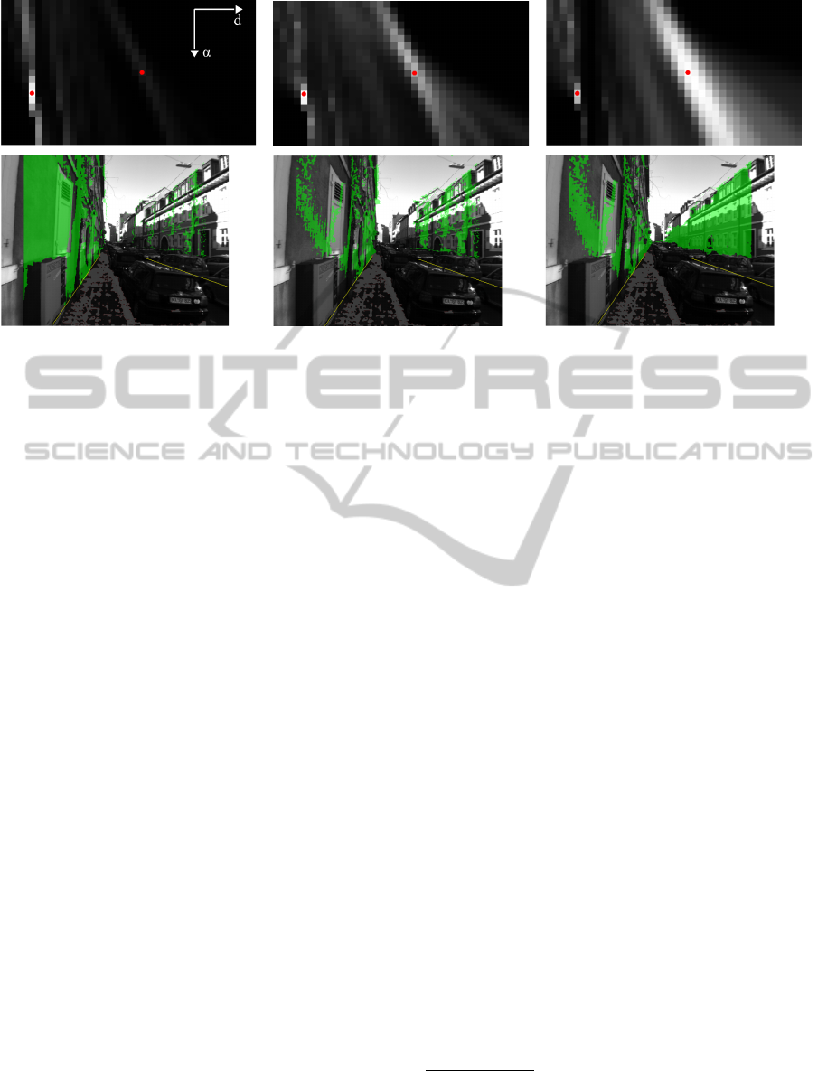
(a) XY Z-points, fixed distance threshold (b) XYZ-points, distance threshold scaled by
covariance
(c) uvδ-points, fixed distance threshold
Figure 1: Plane estimation based on point-to-plane distance thresholds using (a) a fixed distance in XY Z coordinates, (b) the
Mahalanobis distance in XYZ coordinates and (c) a fixed distance in uvδ coordinates. The top row visualizes with gray values
the number of support points for a vertical plane swept through the XYZ- resp. uvδ-points in distance and angle steps of 0.5m
resp. 1
◦
. The true plane parameters are marked in red. The bottom row shows support points for these plane parameters as
overlay.
in connected surfaces when occlusions visually split
the data, a subsequent merging step would be nec-
essary. This does not occur when parametric models
are fitted directly. Most popular methods here are ran-
dom sampling and 3D Hough transformations (Iocchi
et al., 2000).
A large body of literature focuses specifically on
the task of groundplane estimation, in case of vision
systems planes have been extracted using v-disparity
representations (Labayrade et al., 2002) and robust
fitting methods (Se and Brady, 2002), often assum-
ing fixed sensor orientation (Chumerin and Van Hulle,
2008).
We start with estimating the groundplane using
random sampling. Based on the groundplane parame-
ters we constrain the search space to fit two planes to
the left and right building facade. In Section 2.2 and
2.3 we present two robust methods to fulfil this task.
In Section 3 we evaluate both methods using a dataset
of inner city scenes and show how visual odometry
data can be integrated to keep track of the estimated
geometry.
2 PLANE FITTING
Estimating planar structures from an egocentric view-
point in urban environments has to deal with a huge
amount of occlusions. Especially the groundplane is
often only visible in a very small part of the image
since buildings, cars or even pedestrians normally oc-
clude free view onto the ground. Hence, robustness of
the methods is a key requirement. Therefore, we de-
veloped an approach based on the RANSAC scheme
(Fischler and Bolles, 1981), which is known to pro-
duces convincing results on model fitting problems
even with way more than 50% outliers. In a scenario
with fairly free view and cameras pointing towards the
horizon with little tilt a good heuristic is to constrain
the search space to the lower half of the camera image
space to find an initial estimate of the groundplane.
A plane described through the equation
aX +bY + cZ + d = 0
can be estimated using the RANSAC scheme by re-
peatedly selecting 3 random points and evaluating the
support of the plane fitting these points. A fit is eval-
uated by counting the 3D points with point-to-plane
distance less than a certain threshold. In our case,
we had to extend the RANSAC scheme by an adap-
tive threshold to cope with the varying inaccuracy of
3D points determined from a stereo camera. To ac-
count for the uncertainty, the covariance matrices of
the XY Z points can be incorporated into the distance
threshold. In case of reconstructing from stereo vision
one obtains the 3D coordinates (X,Y,Z)
1
through:
1
Our Z-axis equals the optical axis of the camera, X-
axis pointing right and Y-axis towards the ground. Compare
Figure 2
ICINCO2013-10thInternationalConferenceonInformaticsinControl,AutomationandRobotics
84
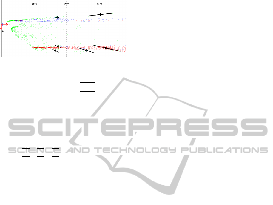
Figure 2: Stereo covariances.
F(u,v,δ) =
X
Y
Z
=
B(u−c
x
)
δ
B(v−c
y
)
δ
B f
δ
(1)
Where B is the baseline, f the focal length, δ
the disparity measurement at image point (u,v), and
(c
x
,c
y
) the principal point. The covariance matrix C
can be calculated by (also found in (Murray and Lit-
tle, 2004)) C = J · M · J
T
with J the Jacobian of F
J =
dF
X
du
dF
X
dv
dF
X
dδ
dF
Y
du
dF
Y
dv
dF
Y
dδ
dF
Z
du
dF
Z
dv
dF
Z
dδ
=
B
δ
0
−B(u−c
x
)
δ
2
0
B
δ
−B(v−c
y
)
δ
2
0 0
−B f
δ
2
Assuming a measurement standard deviation of
1px for the u and v coordinates and a disparity match-
ing error of 0.05px we obtain as measurement matrix
M = diag(1,1,0.05). A world point on the optical
axis of the camera in 15 m distance is subject to a
standard deviation of ∼1 m (focal length 400px, base-
line 12cm). While the Z uncertainty of reconstructed
points grows quadratically with increasing distance,
the uncertainty of reconstructed X and Y components
remains reasonable small (see Figure 2).
With the covariance matrices we can determine
the point to plane Mahalabobis distance and use it in-
stead of a fixed distance threshold to count plane sup-
port points. This way the plane margin grows with in-
creasing camera distance according to the uncertainty
of the reconstruction. Calculating the point to plane
Mahalanobis distance essentially means transforming
the covariance uncertainty ellipses into spheres. A
way to do so is shown in (Schindler and Bischof,
2003).
However, calculating the covariance matrix for ev-
ery XY Z-point is computationally expensive. We can
avoid this by fitting planes in the uvδ-space and trans-
forming the plane parameters into XYZ-space after-
wards.
Fitting planes in uvδ-space can be done in the
same way as described above for the XY Z-space. We
obtain the plane model satisfying the equation
αu + βv + γ −δ = 0
Expressing u,v, δ through equations (1) yields the uvδ
to XY Z-plane transformation
a = α; b = β; c =
αc
x
+ βc
y
+ γ
f
; d = −B
and vice-versa
α =
aB
d
; β =
bB
d
; γ =
B(c f − ac
x
− bc
y
)
d
In the following section we demonstrate the im-
portance of considering the reconstruction uncertainty
when setting the plane distance threshold.
2.1 Sweep Planes
For the purpose of estimating facades of houses we
construct a plane vertical to the groundplane and
sweep it through the XY Z- respectively uvδ-points.
For most urban scenarios it is a valid assumption
that man-made structures and even many weak and
cluttered structures like forest edges or fences are
strongly aligned vertical to the floor. Knowledge of
the groundplane parameters {~n
gp
,d
gp
} with ground-
plane normal ~n
gp
and distance d
gp
from the camera
origin allows us to construct arbitrary planes perpen-
dicular to the ground.
We construct a sweep plane vector perpendicular
to ~n
gp
and the Z-axis (compare Figure 2) by
~n
sweep
(α) = R
~n
gp
(α)
~n
gp
×
0
0
1
,
where rotation matrix R
~n
gp
(α) rotates α degrees
around the axis given by ~n
gp
.
We sweep the plane {~n
sweep
(α),d
sweep
} through
the XY Z respectively uvδ-points by uniformly sam-
pling α and d
sweep
and store the number of sup-
port points for every sample plane in the parameter
space (α,d
sweep
). The result for a sampling between
−10
◦
< α < 10
◦
and −3m < d
sweep
< 15m with a
stepsize of 1
◦
resp. 0.5m is shown in Figure 1. Peaks
in the parameter space correspond to good plane sup-
port.
A fixed threshold in XY Z-space (Figure 1(a))
overrates planes close to the camera (left facade),
while planes further away are underrated (right wall).
The Mahalanobis threshold (Figure 1(b)) can com-
pensate for this. Fitting planes in uvδ-space leads to
the same result (Figure 1(c)), without the computa-
tional expense.
The method can be used to extract planar sur-
faces from the points, regardless whether input data is
present in XY Z- or uvδ-space. It is easy to incorporate
prior scene knowlegde like geometric cues to select
WallEstimationfromStereoVisioninUrbanStreetCanyons
85

planes and suppress non-maxima. Parallel planes are
mapped to the same rows in parameter space, while a
minimal distance between selected planes can be en-
forced by the column gap.
In practice, when knowledge about the rough ori-
entation of the scene is unavailable, the computational
cost of building the parameter space is very high. In
our strongly constrained example scene with ±10
◦
heading angle and 18m distance already 777 planes
had to be evaluated. The required size and subsam-
pling of parameter space is hard to anticipate and
would have to be chosen much bigger, which makes
the approach less attractive in this simple form.
Due to the fact that the plane sweeping is not a
data-driven approach, many planes are evaluated that
are far off the real plane parameters. Simplifying the
data does not affect the number of evaluated planes.
In its data-driven form this algorithm resembles the
Hough transform (Hough, 1962), which has also been
studied and extended for model-fitting problems in
3D data, e.g. (Borrmann et al., 2011).
In the following sections we present two data-
driven approaches for wall estimation. First, we show
how RANSAC can be used to achieve a planar scene
segmentation, from which we extract the street geom-
etry. In Section 2.3 we use a 2D Hough transform to
find the left and right facade.
Figure 3: RANSAC based planar segmentation. The two
most parallel planes (bottom) are selected from five hy-
potheses (top).
2.2 Planar RANSAC Segmentation
RANSAC based plane fitting can obviously not only
be used to fit the groundplane but any other planar
structure in the scene. Assuming the groundplane pa-
rameters are known, we first remove the groundplane
points from uvδ-space. In the remaining points we
iteratively estimate the best plane using RANSAC.
Since we are interested in vertical structures, we can
reject plane hypotheses that intersect the groundplane
at smaller angles than 70
◦
by comparing their nor-
mal vectors. After every iteration we remove the
plane support points from uvδ-space. This way we
generate five unique plane hypotheses, out of which
we select the two most parallel planes with distance
d = |~n
1
d
1
+~n
2
d
2
| > 5m by pairwise comparison to ob-
tain the left and right building facade. Figure 3 shows
an example scene with five plane hypotheses (top) out
of which the red and blue one are selected since they
are the most parallel and also exceed the minimal dis-
tance threshold.
The top row in Figure 4 presents the output for
some challenging scenarios, some of which feature
considerable occlusions. In every iteration we eval-
uate 50 planes with a valid groundplane intersection
angle, 5 iterations hence summing to 250 evaluated
plane hypotheses.
2.3 Elevation Maps
The strong vertical alignment of man-made environ-
ments can be exploited by transforming the 3D point
data into an elevation map. We do this by discretizing
the groundplane into small cells (e.g. 10x10cm) and
projecting the 3D points along the groundplane nor-
mal onto this grid. The number of 3D points project-
ing onto a cell provides a hint about the elevation over
ground for the cell. Grid cells underneath high verti-
cal structures will count more points than grid cells
underneath free-space. Now, the grid can be analysed
using 2D image processing tools. In case of a street
scenario with expected walls left and right we apply
a Hough transform to discover two long connected
building facades. Because of geometric plausibility
we again enforce a minimal distance of 5m between
walls when selecting the Hough peaks. Two examples
along with their elevation map are shown in Figure 5.
The approach also works with weak structures
like forest edges (bottom image), though overhanging
trees are obviously causing a deviation from the real
forest bottom here and the assumed street model with
two walls does not hold in this view. The approach
will benefit strongly from integrating elevation maps
over multiple frames, which is topic of future work.
ICINCO2013-10thInternationalConferenceonInformaticsinControl,AutomationandRobotics
86
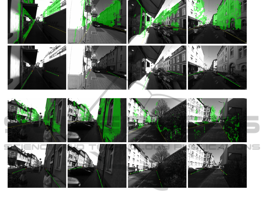
(a) (b) (c) (d)
(e) (f) (g) (h)
Figure 4: Results of RANSAC based planar segmentation (top row) and estimation of facade orientations using elevation
maps (bottom row), which can be used in a subsequent step to generate an according surface.
2.4 Iterative Least-squares
The random nature of the RANSAC segmentation and
the assumption of perfectly vertical buildings in case
of the elevation maps prevent either approach to pro-
duce perfectly robust results. Nevertheless, both ap-
proaches normally yield an approximation of the main
orientation of the buildings, which is accurate enough
to optimize the estimated surface with a least squares
estimator. To deal with the remaining outliers we op-
timize the plane hypotheses iteratively. While shrink-
ing the plane to point distance threshold in every iter-
ation, the optimization converges within a few itera-
tions.
We verify the plane by comparing the normal an-
gle deviation between the initial fit and the optimized
fit. A false initial fit will lead to big deviations and
can be rejected in this way.
3 EXPERIMENTS
In a set of experiments we compare the different
approaches for plane estimation. Our experimental
setup consists of a calibrated stereo rig with a short
baseline of around 10 cm and a video resolution of
640x480px. To enlarge the field-of-view we deploy
a wide-angle lens of 12 mm focal length. We obtain
the dense disparity estimation using an off-the-shelf
semi-global-matching approach (OpenCV).
3.1 Evaluation
We ran some tests on a dataset consisting of inner city
scenes captured from ego-view to evaluate the appli-
cability of the proposed approaches in some challeng-
ing scenarios. Processing video data from ego-view
perspective especially has to be robust against occlu-
sion and the high degree of clutter caused by parked
cars or bikes, trees, or other dynamic traffic partici-
pants. Another issue in real life scenarios are the chal-
WallEstimationfromStereoVisioninUrbanStreetCanyons
87
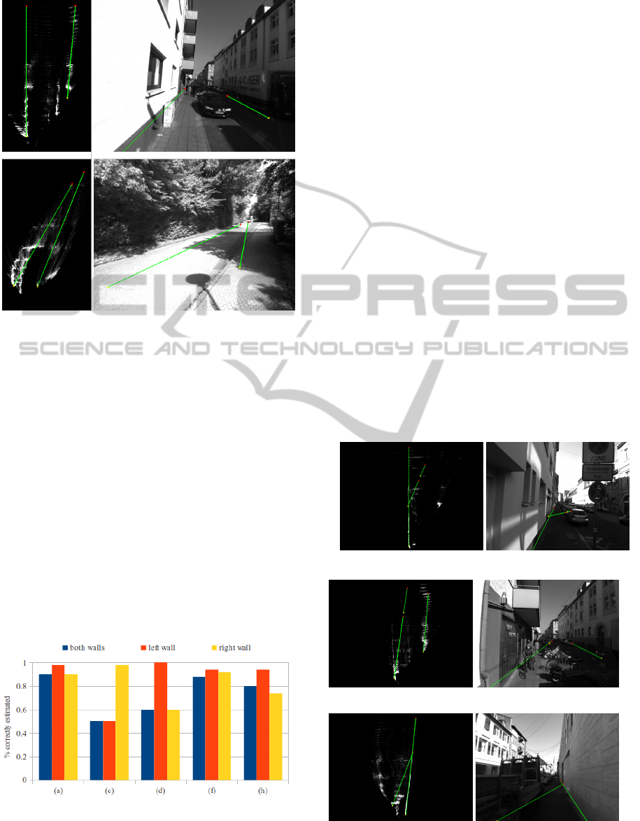
Figure 5: Left column: Elevation maps. Connected el-
ements are found by Hough transformation and projected
into the camera image (right column).
lenging light conditions, that often lead to over- and
underexposed image parts in the same image. Figure
4 shows 8 scenes with the result of RANSAC segmen-
tation in the top row, and the resulting facade orienta-
tion drawn from elevation maps in the bottom row.
Planar RANSAC Segmentation
The random plane selection in the RANSAC segmen-
tation approach makes it difficult to draw quantita-
tive conclusions about the performance. To underlay
some numbers we picked five of the more difficult
scenarios and evaluated the repeatability of the out-
put. We ran the algorithm 50 times on each scenario
and evaluated the number of correct wall estimations
by manual supervision. We consider a wall as missed
Figure 6: Evaluation of repeatability of planar RANSAC
segmentation. Shown is the percentage of correctly deter-
mined walls in 50 repetitions, scenes correspond to Fig-
ure 4.
when the estimated orientation deviates so strongly,
that a subsequent optimization step will not converge
close to the optimum.
Figure 6 shows the results for some scenarios
taken from Figure 4. Scenario (c) is challenging in
that the left building wall is hardly visible due to oc-
clusion, and the visible part is overexposed. The right
wall is found very robustly. The large amount of er-
rors in detecting the right wall in scenario (d) can be
explained by clutter, which often leads to planes fitted
to the sides of the parked cars. Increasing the number
of sampled planes per iteration would probably pre-
vent this. The substantial gap on the right hand side
in (h) explains the often missed right wall. In scenar-
ios with mostly free view on the walls a rate of around
90% for both walls is realistic.
Elevation Maps
To rate the stability of wall estimation based on el-
evation maps we investigate two sequences of 200
and 500 frames, taken while travelling down a street
canyon. In each frame we estimate the orientation of
both walls, independent of the previous frame.
The first sequence consists of 200 frames and is
mostly free of wall occlusions. The algorithm finds
the correct wall orientation in all but 8 frames, that
(a)
(b)
(c)
Figure 7: Failures in orientation estimation using elevation
maps.
ICINCO2013-10thInternationalConferenceonInformaticsinControl,AutomationandRobotics
88
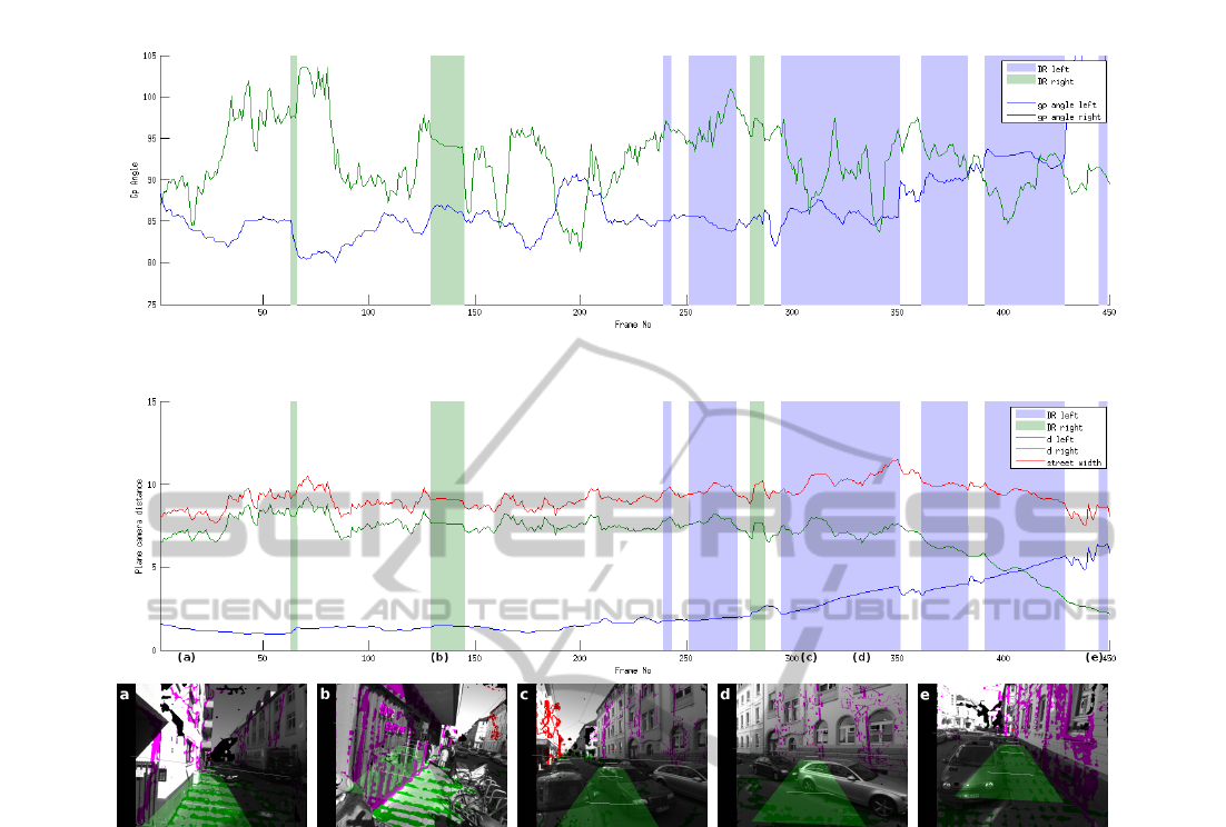
Figure 8: Plane parameters tracked over a sequence of 450 frames. The top diagram shows the groundplane angle, the bottom
diagram the normal plane distance. Predicted parts due to walls being out of view are shaded.
were taken while passing a street sign (see Figure
7(a)). The second sequence consists of 500 frames
and is more cluttered. The algorithm fails in around
10% of all frames to estimate one of the walls cor-
rectly. Reasons are always related to obstacles that
were not filtered because they exceed the groundplane
cut-off height, or obstacles that occlude the wall. See
Figures 7(b) and 7(c) for two examples.
3.2 Geometry Tracking
The wall estimation is embedded as part of a real-
time system, which also contains a module to esti-
mate the camera motion between consecutive frames
by running the visual odometry estimation taken from
the LIBVISO2 library (Geiger et al., 2011b). Visual
odometry provides the egomotion in all six degrees of
freedom such that the camera poses of frame n−1 and
n are related via a translation vector
~
t and a rotation
matrix R.
Knowledge of the camera transformation allows
to predict the current groundplane and wall param-
eters from the previous frame. The XYZ-plane
~p
t−1
= {~n,d}, with surface normal ~n and distance d
from the camera origin, transforms into the current
frame via
~p
t
=
[R|
~
t]
−1
T
~p
t−1
In a street canyon scenario we proceed as follows:
We initialize the groundplane and planes for left and
right wall with the methods described above. For
the following frames we use the prediction as start-
ing point for the iterative least squares optimization
to compensate the inaccuracy of the egomotion esti-
mation. To stabilize the process over time we store
the best fitting support points in a plane history ring
buffer and incorporate them with a small weighting
factor into the subsequent least squares optimization.
We reject the optimization when the plane normal an-
gles of prediction and optimization deviate by more
than 5
◦
in either direction, or the groundplane angle
becomes smaller than 80
◦
. Reasons for this to hap-
WallEstimationfromStereoVisioninUrbanStreetCanyons
89

pen are normally related to a limited view onto the
wall, which either occurs when the wall is occluded
by some close object (e.g. truck), or the cameras tem-
porarily point away from the wall. If the optimiza-
tion was rejected we carry over the prediction as cur-
rent estimate and continue like that until the wall is in
proper view again.
The estimated plane parameters for both walls in a
sequence over 450 frames are plotted in Figure 8. The
upper diagram shows the angle between groundplane
and walls, the bottom diagram shows the plane dis-
tance parameters. The distances add up to the street
width, for this sequence with a mean of 9.3m.
The sequence begins on the left sidewalk and ends
on the right sidewalk after crossing the street. It con-
tains several parts in which the walls are out of view
due to the camera heading, some are shown in the
screen shots. As explained earlier, these parts are
bridged by predicting the parameters using the ego-
motion and are shaded in the diagram.
4 CONCLUSIONS
We have demonstrated two approaches towards esti-
mating the local, geometric structure in the scenario
of urban street canyons. We model the right and left
building walls as planar surfaces and estimate the un-
derlying plane parameters from 3D data points ob-
tained from a passive stereo-camera system, which is
replaceable by any kind of range sensor as long the
uncertainties of reconstructed 3D points are known
and can be considered.
The presented approaches are not intended as a
standalone version. Their purpose is rather to separate
a set of inlier points fitting the plane model to initial-
ize optimization procedures as we applied in form of
the iterative least-squares. By taking visual odometry
in combination with a prediction and update step into
the loop we are able to present a stable approach to
keep track of groundplane and both walls.
Future work includes integrating the rich informa-
tion offered by the depth-registered image intensity
values and relaxing the assumptions implied by the
street canyon scenario.
ACKNOWLEDGEMENTS
The work was supported by the German Federal Min-
istry of Education and Research within the project
OIWOB. The authors would like to thank the
”Karlsruhe School of Optics and Photonics” for sup-
porting this work.
REFERENCES
Barinova, O., Lempitsky, V., Tretiak, E., and Kohli, P.
(2010). Geometric image parsing in man-made en-
vironments. ECCV’10, pages 57–70, Berlin, Heidel-
berg. Springer-Verlag.
Borrmann, D., Elseberg, J., Lingemann, K., and N
¨
uchter, A.
(2011). The 3d hough transform for plane detection in
point clouds: A review and a new accumulator design.
3D Res., 2(2):32:1–32:13.
Chumerin, N. and Van Hulle, M. M. (2008). Ground Plane
Estimation Based on Dense Stereo Disparity. ICN-
NAI’08, pages 209–213, Minsk, Belarus.
Cornelis, N., Leibe, B., Cornelis, K., and Gool, L. V.
(2008). 3d urban scene modeling integrating recog-
nition and reconstruction. International Journal of
Computer Vision, 78(2-3):121–141.
Fischler, M. A. and Bolles, R. C. (1981). Random sample
consensus: a paradigm for model fitting with appli-
cations to image analysis and automated cartography.
Commun. ACM, 24(6):381–395.
Geiger, A., Lauer, M., and Urtasun, R. (2011a). A gen-
erative model for 3d urban scene understanding from
movable platforms. In CVPR’11, Colorado Springs,
USA.
Geiger, A., Ziegler, J., and Stiller, C. (2011b). Stereoscan:
Dense 3d reconstruction in real-time. In IEEE Intelli-
gent Vehicles Symposium, Baden-Baden, Germany.
Gutmann, J.-S., Fukuchi, M., and Fujita, M. (2008).
3d perception and environment map generation for
humanoid robot navigation. I. J. Robotic Res.,
27(10):1117–1134.
Hoiem, D., Efros, A. A., and Hebert, M. (2007). Recovering
surface layout from an image. International Journal
of Computer Vision, 75:151–172.
Hoover, A., Jean-baptiste, G., Jiang, X., Flynn, P. J., Bunke,
H., Goldgof, D., Bowyer, K., Eggert, D., Fitzgibbon,
A., and Fisher, R. (1996). An experimental compari-
son of range image segmentation algorithms.
Hough, P. (1962). Method and Means for Recognizing
Complex Patterns. U.S. Patent 3.069.654.
Iocchi, L., Konolige, K., and Bajracharya, M. (2000). Vi-
sually realistic mapping of a planar environment with
stereo. In ISER, volume 271, pages 521–532.
Labayrade, R., Aubert, D., and Tarel, J.-P. (2002). Real
time obstacle detection in stereovision on non flat road
geometry through ”v-disparity” representation. In In-
telligent Vehicle Symposium, 2002. IEEE, volume 2,
pages 646 – 651 vol.2.
Lee, D. C., Hebert, M., and Kanade, T. (2009). Geomet-
ric reasoning for single image structure recovery. In
CVPR’09.
Murray, D. R. and Little, J. J. (2004). Environment model-
ing with stereo vision. IROS’04.
Poppinga, J., Vaskevicius, N., Birk, A., and Pathak, K.
(2008). Fast plane detection and polygonalization in
noisy 3d range images. IROS’08.
Schindler, K. and Bischof, H. (2003). On robust regression
in photogrammetric point clouds. In Michaelis, B. and
Krell, G., editors, DAGM-Symposium, volume 2781 of
Lecture Notes in Computer Science, pages 172–178.
Springer.
Se, S. and Brady, M. (2002). Ground plane estimation, error
analysis and applications. Robotics and Autonomous
Systems, 39(2):59–71.
ICINCO2013-10thInternationalConferenceonInformaticsinControl,AutomationandRobotics
90
