A Flexible Framework for Mobile Robot Pose Estimation
and Multi-Sensor Self-Calibration
Davide Antonio Cucci and Matteo Matteucci
Dipartimento di Elettronica, Informazione e Bioingegneria, Politecnico di Milano, Milan, Italy
Keywords:
Sensor Fusion, Mobile Robots, Odometry, Tracking, Calibration.
Abstract:
The design and the development of the position and orientation tracking system of a mobile robot, and the
calibration of its sensor parameters (e.g., displacement, misalignment and iron distortions), are challeng-
ing and time consuming tasks in every autonomous robotics project. The ROAMFREE framework delivers
turn-on-and-go multi-sensors pose tracking and self-calibration modules and it is designed to be flexible and
to adapt to every kind of mobile robotic platform. In ROAMFREE, the sensor data fusion problem is for-
mulated as a hyper-graph optimization where nodes represent poses and calibration parameters and edges the
non-linear measurement constraints. This formulation allows us to solve both the on-line pose tracking and
the off-line sensor self-calibration problems. In this paper, we introduce the approach and we discuss a real
platform case study, along with experimental results.
1 INTRODUCTION
In every project involving autonomous robots the de-
sign and development of the pose tracking subsys-
tem is one of the first and most important mile-
stones (Borenstein et al., 1996). This task is often
time consuming and the performance of higher level
control and navigation modules are tightly dependent
on the localization accuracy. Moreover, to determine
an estimate of the robot position and attitude with re-
spect to the world, multiple sensors are usually em-
ployed. This often requires the calibration of intrin-
sic parameters for which direct measurement is im-
practical or impossible and the calibration task is usu-
ally performed by mean of time consuming ad-hoc,
hand-tuned procedures especially designed to target
the platform in use.
The ROAMFREE project aims at developing a
general framework for robust sensor fusion and self-
calibration to provide a turn-on-and-go 6-DOF pose
tracking system for autonomous mobile robots. It in-
cludes: (i) a library of sensor families which are han-
dled by the framework out-of-the box; (ii) an on-line
tracking module based on Gauss-Newton minimiza-
tion of the error functions associated to sensor read-
ings; (iii) an off-line calibration suite which allows to
estimate unknown sensor parameters such as the dis-
placement and the misalignment with respect to the
robot odometric center, scale factors and biases, mag-
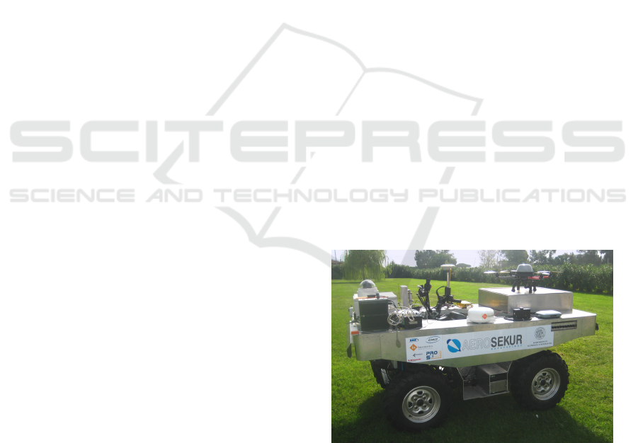
Figure 1: The Quadrivio ATV.
netometer soft and hard iron distortion, and so on.
In the mobile robots literature the position and ori-
entation tracking problem has often been addressed
as a problem of multi-sensor data fusion and solved
by means of Bayesian filters, such as Kalman and
particle filters (Chen, 2003). Bayesian filtering has
also been employed to the problem of on-line estima-
tion of calibration parameters, such as the systematic
and non-systematic components of the odometry er-
ror (Martinelli et al., 2007), or quantities which af-
fects the tracking performances, such as the GPS la-
tency (Bouvet and Garcia, 2000). If we restrict to the
off-line calibration of single sensor displacement and
misalignment, the problem is commonly referred as
hand-eye clibration (Horaud and Dornaika, 1995).
361
Antonio Cucci D. and Matteucci M..
A Flexible Framework for Mobile Robot Pose Estimation and Multi-Sensor Self-Calibration.
DOI: 10.5220/0004484703610368
In Proceedings of the 10th International Conference on Informatics in Control, Automation and Robotics (ICINCO-2013), pages 361-368
ISBN: 978-989-8565-71-6
Copyright
c
2013 SCITEPRESS (Science and Technology Publications, Lda.)
Although the effectiveness of previous approaches
has been proven and are now well established in the
literature, researchers are still required to write their
own on ad-hoc implementations to adapt state-of-the-
art techniques to the particular application or plat-
form. More recently, in (Weiss et al., 2012), a general
framework for position tracking and sensor displace-
ment calibration is presented which relies on an Ex-
tended Kalman Filter to perform sensor fusion tasks.
Similarly, our work focuses on the development of
a very general framework suited to be employed in ev-
ery kind of autonomous robot platform. In this paper
we describe the first deployment of the system to tar-
get the Quadrivio ATV, (see Figure 1), an autonomous
off-road vehicle equipped with a wide variety of sen-
sors, such as laser rangefinders, GPS, wheel and han-
dlebar encoders and an Inertial Measurement Unit,
which have to be integrated and calibrated to deliver
6-DOF position and orientation estimate to the higher
level trajectory control and navigation modules. Dif-
ferently from (Weiss et al., 2012), we base our frame-
work on the use of a Gauss-Newton graph based esti-
mation techniques as the ones applied in (K
¨
ummerle
et al., 2012) to the problem of 3-DOF simultaneous
localization, mapping and calibration.
In the next section we give a high level descrip-
tion of the ROAMFREE framework; in Section 3 and
Section 4 we go more in depth in the techniques em-
ployed and we describe the mathematical background
that allows to perform the data fusion task in a sensor
independent manner. In Section 5 we present the first
deployment of the framework on the Quadrivio ATV
and discuss preliminary experimental results. Con-
clusions and further work appear in Section 6.
2 FRAMEWORK DESCRIPTION
The ROAMFREE framework is designed to fuse dis-
placement measurements coming from an arbitrary
number of odometric sensors. Here, we focus on the
generality of the approach trying to abstract as much
as possible from the nature of the information sources.
To this ends, we choose not to work directly with
physical hardware, but with logical sensors, which are
characterized only by the type of the proprioceptive
measurement they produce. To clarify this point, con-
sider a SLAM system built on the top of wheel en-
coders and multiple cameras. We call logical sensor
the set of the encoders, the cameras and the SLAM
algorithm, since, ultimately, it estimates the absolute
pose of the robot with respect to a fixed reference
frame. Moreover, the wheel encoders, taken alone,
build up another logical sensor which measures the
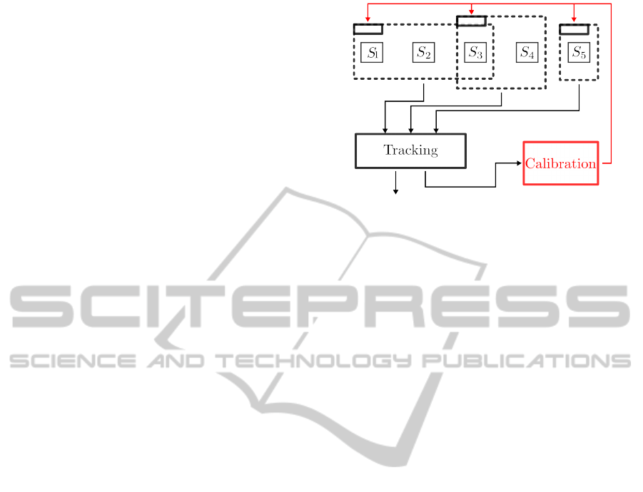
Figure 2: The ROAMFREE logical structure. Eventually
overlapping groups of physical sensors, S
i
, build up logical
information sources whose output is fused by the tracking
module. The position and attitude output is employed off-
line by the calibration module to estimate intrinsic parame-
ters of the logical sensors.
roto-translation between poses at time t and t + ∆t.
ROAMFREE allows the end-user to define logical
sensors building up on separate modules and automat-
ically integrate their measurements to both obtain a
robust estimate of the robot pose and to calibrate un-
known sensor parameters (see Figure 2). In this way,
the developer can focus only on the internals of each
logical sensor (e.g., signal processing, visual odom-
etry algorithms), which extract information from the
raw sensor data and then deliver it to ROAMFREE,
e.g. through ROS (Quigley et al., 2009).
To achieve the abstraction form the physical
hardware and be able to deal with very gen-
eral, user-defined, information sources we ob-
serve that, despite the wide variety of proprio-
ceptive sensors available for the design of mobile
robots, all the useful logical sensor output for pose
tracking fit into one of the following categories:
• absolute position and/or velocity
• angular and tangential speed in sensor frame
• acceleration in sensor frame
• vector field in sensor frame (e.g., magnetic field,
gravitational acceleration)
For each of these categories ROAMFREE provides an
error model which relates the state estimate with the
measurement data, taking into account all the com-
mon sources of distortion, bias and noise (e.g., hard
and soft magnetic distortion, sensor displacement or
misalignment, etc.). These error models are then em-
ployed in the on-line estimation process to handle
the logical sensor readings, according to their type.
Moreover, the final user can choose a set of the pre-
defined calibration parameters for which he can either
provide values or let the framework estimate them us-
ICINCO2013-10thInternationalConferenceonInformaticsinControl,AutomationandRobotics
362
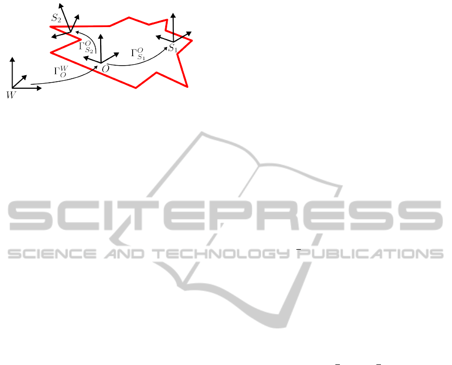
Figure 3: The reference frames employed in ROAMFREE.
To represent the odometric reference frame O we store
Γ
W
O
= [O
(W )
,q
W
O
]. The sensor displacements and misalign-
ment parameters of sensor S
i
define the roto-translation
from the odometric reference frame to the S
i
reference
frame Γ
O
S
i
= [S
(O)
i
,q
O
S
i
].
ing an off-line formulation of the tracking problem.
In the following, a reference frame A will be rep-
resented with the roto-translation Γ
B
A
which takes a
point p
(A)
, whose coordinates are expressed in refer-
ence frame A, to reference frame B. To represent such
transformations, we use the origin of A expressed in
reference frame B, A
(B)
, and the quaternion q
B
A
, i.e.,
the rotation taking points from frame A to frame B.
So Γ
B
A
= [A
(B)
,q
B
A
].
ROAMFREE makes use of three reference frames
(see Figure 3): W, the fixed world frame, O, the mov-
ing reference frame, placed at the odometric center
of the robot, and the i-th sensor frame, S
i
, whose ori-
gin and orientation are defined with respect to O in
terms of displacement and misalignment. The track-
ing module estimates the position and orientation of
O with respect to W , i.e., Γ
W
O
. If absolute positioning
sensors (e.g., GPS) are not available, we assume that
O ≡ W at time t = 0, and W becomes arbitrary. Oth-
erwise, the origin of W is placed at given coordinates,
with the y axis aligned with the geographic north and
the z axis aligned with g and pointing up.
Currently we assume that all the logical sensor
readings are precisely timestamped and that all the
clocks in the system are synchronized. The impor-
tance of accurate measurement timestamps has been
often stressed in the literature and a number of clock
synchronization algorithms designed for robotics ap-
plications exist, i.e., (Harrison and Newman, 2011).
If accurate timestamps are available, the framework
is robust with respect to out-of-order measurements,
as it will become clear in the next section.
The ROAMFREE framework is open-source and
it is available at http://roamfree.dei.polimi.it.
3 POSE TRACKING AND
SENSOR SELF-CALIBRATION
We formulate the tracking problem as a maximum
likelihood optimization on an hyper graph in which
the nodes represent poses and sensor parameters (to
be eventually estimated) and hyper-edges correspond
to measurement constraints. An error function is as-
sociated to each hyper-edge to measure how well the
values of the nodes involved in the hyper-edge fit the
sensor observations. The goal of the max-likelihood
approach is to find a configuration for the poses and
sensor parameters which minimizes the negative log-
likelihood of the graph given all the measurements.
Let us discuss more precisely the problem for-
mulation and techniques employed to solve it. Let
e
i
(x
i
,η) be the error function associated to the i-th
edge in the hyper graph, where x
i
is a vector contain-
ing the variables appearing in any of the connected
nodes and η is a zero-mean Gaussian noise. Thus
e
i
(x
i
,η) is a random vector and its expected value
is computed as e
i
(x
i
) = e
i
(x
i
,η)|
η=0
. Since e
i
can
involve non-linear dependencies with respect to the
noise vector, we compute the covariance of the error
through linearization. Let Σ
η
be the covariance matrix
of η and J
i
the Jacobian of e
i
with respect to η:
Σ
e
i
= J
i
Σ
η
J
T
i
η=0
. (1)
The optimization problem is defined as follows:
P : argmin
x
N
∑
i=1
e
i
(x
i
)
T
Ω
e
i
e
i
(x
i
), (2)
where Ω
e
i
= Σ
−1
e
i
is the i-th edge information matrix
and N is the total number of edges. If a reasonable ini-
tial guess for x is known, a numerical solution for P
can be found by means of the poular Gauss-Newton
(GN) or Levenberg-Marquardt (LM) algorithms, see
for example (Gill and Murray, 1978): first the error
functions are approximated with their first order Tay-
lor expansion around the current estimate ˘x:
e
i
( ˘x ∆x) ' e
i
( ˘x) +J
i
∆x, (3)
where J
i
is the Jacobian of e
i
with respect to ∆x eval-
uated in ∆x = 0 and is an operator which applies
an increment ∆x to ˘x. Substituting the error functions
e
i
(x
i
) in (2) with their first order expansion yields a
quadratic form which can be solved in ∆x. Finally we
set ˘x ← ˘x ∆x and we update the Ω
e
i
as in (1). The
process is iterated till termination criteria are met.
Note that this formulation of the optimization
problem, thanks to the operator, allows us to
consistently work with variables which span over
non-Euclidean spaces, such as SO(3) and SE(3).
AFlexibleFrameworkforMobileRobotPoseEstimationandMulti-SensorSelf-Calibration
363

In these cases, over-parametrized representations are
often employed, and substituting the operator
with regular + in (3) would yield solutions for
∆x which could break the constraints induced by
over-parametrization. Instead, the operator con-
sistently applies a local variation ∆x, belonging to an
Euclidean space, to the original variable. Consider for
instance x being a quaternion: a 4D representation is
employed to represent 3-DOF rotations.
x ∆x = x ⊗
1 −
q
∆x
2
1
+ ∆x
2
2
+ ∆x
2
3
,∆x
1
,∆x
2
,∆x
3
,
(4)
where ⊗ is the quaternion product operator and ∆x ∈
ℜ
3
. This ensures that ||x ∆x|| = 1 and that quater-
nions are consistently updated once ∆x has been de-
termined. This technique is called manifold encapsu-
lation, for details see (Hertzberg et al., 2013).
We next discuss how an instance of the hyper-
graph optimization problem for the tracking and/or
sensor self-calibration problem is constructed (see
Figure 4). We first need to instantiate pose and pa-
rameter nodes and measurement edges and then de-
termine an initial guess for all the variables in the
problem. We choose a high frequency sensor from
which it is possible to predict Γ
W
O
(t +∆t) given Γ
W
O
(t)
and its measurement z(t). Each time a new read-
ing for this sensor is available, we instantiate a new
node Γ
W
O
(t + ∆t) using the last pose estimate avail-
able,
˘
Γ
W
O
(t), and z(t) to compute an initial guess for
this node. z(t) is also employed to initialize an odom-
etry edge between poses at time t and t + ∆t.
When other measurements from different sensors
are available, their corresponding edge is inserted into
the graph relying on the existing nodes. More pre-
cisely, the pose node (or the pair of poses) nearest
to the measurement timestamp is employed. For in-
stance, if a new gyroscope reading is available with
timestamp t we search in the graph for the pair of sub-
sequent poses with timestamps nearest to t and we in-
sert an angular speed constraint between the selected
nodes. We assume here that, if the sensor employed to
initialize the pose nodes has a sufficiently high sam-
pling rate, the error introduced by this approxima-
tion is negligible. Note that, if the timestamps satisfy
the assumptions mentioned in the previous section,
this approach natively allows to deal with out-of-order
measurements since constraints can be instantiated in
the past between proper pose nodes an contribute to
the refinement of the newest pose estimate.
To solve the optimization problem we employ
g
2
o (K
¨
ummerle et al., 2011), a general framework for
graph optimization which relies on very efficient im-
plementations and it is reported to solve graph prob-
lems with thousands of nodes in fractions of a second,
Figure 4: An instance of the tracking optimization prob-
lem with four pose vertices Γ
W
O
(t) (circles), odometry edges
e
ODO
(triangles), two shared calibration parameters vertices
k and φ (squares), two GPS edges e
GPS
and the GPS dis-
placement S
(O)
GPS
.
allowing us to perform the tracking task on-line.
The graph optimization approach is suited to both
the on-line position tracking problem, in which the re-
quirements are substantially related to precision and
robustness of the estimate and real-time frequency
of operation, and the off-line calibration problem, in
which the goal is to determine the sensor parameters
assignments which globally maximize the likelihood
of all the measurements collected during a long robot
roam. Indeed, in case of on-line tracking the param-
eter values are known and the corresponding nodes
are excluded from the optimization. Moreover, to al-
low real time operation, we assume that the process
memory extends up to N time slots in the past and we
discard older nodes and edges. The optimization is
run at constant frequency and we iterate the GN algo-
rithm till timing deadlines approach or when the error
function improvement drops below the chosen thresh-
old. Conversely, during off-line calibration, a set of
the parameter nodes is chosen for estimation and the
graph containing all available measurements is con-
sidered. Note that with the same problem formulation
it is also possible to track on-line a limited set of cal-
ibration parameters, along with the robot pose, which
are subject to change, such as slippage coefficients.
4 ERROR MODELS
In this section we introduce the sensor models em-
ployed in ROAMFREE and the corresponding error
functions, which measure how well the sensor read-
ing fit the corresponding poses. Since error functions
are evaluated multiple times during GN optimization,
when we refer to state variables, e.g., Γ
W
O
(t), we al-
ICINCO2013-10thInternationalConferenceonInformaticsinControl,AutomationandRobotics
364

ways intend their current estimate, e.g.,
˘
Γ
W
O
(t). Sen-
sor parameters are highlighted by a bold font.
4.1 General Odometer
Every kind of odometer can be seen as a sensor which
measures the roto-translation between two subsequent
poses, i.e., Γ
O(t)
O(t+∆t)
, from which, assuming constant
speed between t and t + ∆t, it is possible to obtain
estimates of the robot tangential speed and turn rate
ˆv
(S)
(t) and
ˆ
ω
(S)
(t) in sensor frame. Integrating these
quantities over ∆t yields a predictor for Γ
W
O(t+∆t)
:
ˆ
O
(W )
(t +∆t) =
q
W
O
(t)q
O
S
ˆv
(S)
(t)∆t + O
(W )
(t)
ˆq
W
O
(t +∆t) = Φ
q
O
S
ˆ
ω
(S)
(t), ∆t
q
W
O
(t).
(5)
Here ˆq
W
O
(t + ∆t) it is obtained by means of the well
known Rodriguez formula:
Φ(ω,∆t) =
h
cos(|ω|
∆t
2
)I + 2
sin(|ω|
∆t
2
)
|ω|
W (ω)
i
, (6)
where W (ω) is the 4× 4 skew-symmetric matrix con-
structed from the augmented ω vector [0,ω
x
,ω
y
,ω
z
].
Note that ˆv
(S)
(t) and
ˆ
ω
(S)
(t) are random vectors.
The difference between state estimate and predic-
tors yields the odometry error:
e
ODO
(t) =
ˆ
O
(W )
(t +∆t) − O
(W )
(t +∆t)
ˆq
W
O
(t +∆t) ⊗ [q
W
O
(t +∆t)]
−1
. (7)
Note that the Gaussian noise corrupting
ˆ
ω
(S)
(t), be-
cause of the constraints involved in the quaternion
representation of 3-DOF rotations (i.e., ||q|| = 1),
yields a singular covariance matrix for the full quater-
nion error vector. To overcome this issue, we assume
the orientation error being small (i.e., the quater-
nion part of the error vector is near to the identity,
q ' [1,0,0,0]) and we discard the first component,
yielding a well defined information matrix Ω
e
i
.
Note that a wide variety of sensors can be treated
in this way, e.g., visual odometry systems, scan-
matching algorithms, but also cinematic models,
since a prediction
ˆ
Γ
O(t)
O(t+∆t)
can be computed apply-
ing the forward cinematic to the control inputs. For
the sake of clarity we develop here an example of cin-
ematic odometry based on the platform of Figure 1.
Four wheel vehicles usually employ the Acker-
mann steering geometry. The odometry for these ve-
hicles is computed placing a reference frame S
ACK
in
the middle point of the rear wheels axis. A first or-
der approximation of the dynamic equations govern-
ing the motion of such vehicles yields the predictors
ˆv
(S
ACK
)
(t) and
ˆ
ω
(S
ACK
)
(t) as a function of rear wheels
speed v
ACK
(t) and steering angle θ
ACK
(t), i.e.:
ˆv
(S
ACK
)
(t) =
k
v
v
ACK
(t)
0
0
+ η
v
ˆ
ω
(S
ACK
)
(t) =
0
0
k
v
v
ACK
(t)
L
tan
k
θ
θ
ACK
(t) + k
γ
+ η
ω
,
(8)
where [k
v
,k
θ
,k
γ
] is a vector of gains and biases and L
is the distance between front and rear wheel axes (Abe
and Manning, 2009). Note that the vehicle motion is
constrained on a 2D surface, which is not necessar-
ily flat. The predicted pitch and roll speed are zero,
although these components speed can not be com-
puted with the information provided by v
ACK
(t) and
θ
ACK
(t). Thus we have to consider large variances of
the corresponding components of η.
4.2 GPS
The GPS sensor measures its own latitude, longitude
and elevation with respect to a standard, Earth fixed,
reference frame. The pose of the robot can be em-
ployed to predict the GPS reading, once this has been
projected on an Euclidean ENU (East, Nord, Up)
three-dimensional space centered at W
ˆz
GPS
(t) = O
(W )
(t) + q
W
O
(t)S
(O)
GPS
+ η, (9)
where S
(O)
GPS
is GPS sensor displacement. The same
equation can also be employed with other absolute
positioning logical sensors, such as SLAM systems.
The error associated to the GPS measure is simply
e
GPS
(t) = ˆz
GPS
(t) − z
GPS
(t) and e
GPS
(t) ∈ ℜ
3
.
4.3 Magnetometer
The three-axis magnetometer reading is a measure of
the the Earth’s magnetic field h
(W )
in sensor frame, af-
fected by various sources of distortion, bias and noise.
Here we employ an error model that keeps into ac-
count hard and soft iron distortion, non-orthogonality
of the sensor axes, scaling, bias and misalignment
with respect to the odometric reference frame, as dis-
cussed in (Vasconcelos et al., 2011):
ˆ
z
MAG
(t) = A
q
W
O
(t)q
O
S
MAG
h
(W )
+ b + η, (10)
where A is an unconstrained 3 × 3 matrix, b ∈ ℜ
3
is a bias vector, and h
(W )
is the Earth’s magnetic
field vector in the robot operation area. The error
associated to the magnetometer measurement is then
e
MAG
(t) = ˆz
MAG
(t) − z
MAG
(t) and e
MAG
(t) ∈ ℜ
3
.
AFlexibleFrameworkforMobileRobotPoseEstimationandMulti-SensorSelf-Calibration
365

4.4 Gyroscope
The gyroscope sensor measures its own angular ve-
locity in sensor frame. Here we assume the robot to
be a rigid body and thus experiencing the same angu-
lar velocity at every point. Under this assumption, a
gyroscope provides a direct measure for the angular
velocity of the odometric reference frame. As in (5):
ˆq
W
O
(t +∆t) = Φ
q
O
S
GY RO
(z
GY RO
+ η),∆t
q
W
O
(t), (11)
where the gyroscope reading is moved in the odomet-
ric reference frame by means of the misalignment ro-
tation q
O
S
and then employed to predict robot orien-
tation at time t + ∆t. Thus e
GY RO
can be computed
as the difference between ˆq
W
O
(t + ∆t) in (11) and the
current estimate of q
W
O
(t +∆t):
e
GY RO
(t) = ˆq
W
O
(t +∆t) ⊗ [q
W
O
(t +∆t)]
−1
. (12)
Again we assume that e
GY RO
represents a small rota-
tion and we discard the first component of the quater-
nion so that e
GY RO
∈ ℜ
3
.
5 EXPERIMENTAL RESULTS
In this section we discuss preliminary experimental
results for the first deployment of the ROAMFREE
framework, targeting the Quadrivio ATV (Bascetta
et al., 2009)(Bascetta et al., 2012), an all-terrain au-
tonomous vehicle being developed with the aim of
off-road autonomous navigation on rough terrains. In
these environments, high level navigation and trajec-
tory control modules could benefit from the ROAM-
FREE 6-DOF pose tracking capabilities.
The ATV is equipped with a wide variety of sen-
sors which make it an interesting experimental plat-
form for multi-sensor fusion techniques. These con-
sist in a Xsens MTi, a MEMS inertial measurement
unit with integrated 3D magnetometer, a low cost
Yuan10 L1 C/A code USB GPS receiver and two Sick
laser rangefinders, which were not employed in this
preliminary experiments. Moreover, two encoders
read the handlebar steering angle and wheel speed.
On this platform, we tested the tracking and cal-
ibration capabilities of the ROAMFREE framework.
Indeed, multiple unknown parameters have to be de-
termined in order to achieve maximum pose tracking
accuracy and their direct measurement is not always
simple or practical. Here we focus on the following
set of parameters: the GPS displacement, S
(O)
GPS
and
the Xsens misalignment, q
O
S
IMU
, with respect to the
odometric reference frame, the magnetometer hard
and soft iron distortion compensation matrix and bias,
A and b, the Ackermann steering geometry and en-
coders parameters, [k
v
,k
θ
,k
γ
,L]. We start from raw
sensors data collected while driving the ATV and then
we perform the off-line optimization to find the pa-
rameter values which maximize the likelihood of the
collected measurements.
Note that it is not guaranteed that all the calibra-
tion parameters are observable. For example the z
component of S
(O)
GPS
can not be estimated consider-
ing only planar trajectories. Fortunately, these phe-
nomena can be detected looking at the approximated
Hessian of the error functions computed during the
Gauss-Newton optimization process, from which we
can extract an estimation of the marginal covariance
of the estimates. In case of non-observable parame-
ters given the trajectory considered, their covariance
will be high, implying that perturbations in their val-
ues have limited effect on the error functions. It is
difficult to give theoretical results on the conditions
which have to be satisfied by the trajectory to be able
to observe all of a given set of calibration parame-
ters in the general case. A detailed analysis of the
differential drive case can be found in (Censi et al.,
2008). Morover, multiple solutions to the calibration
problem may exist. Again, these situations can be de-
tected looking at the marginal cross covariance of the
parameter variables, in which high values suggest the
existence of dependencies between the involved pa-
rameters. In these cases one possible strategy is to
first obtain a coarse-grained estimate of one set of pa-
rameters while keeping the dependent ones fixed. In
ROAMFREE this can be done by means of a graphi-
cal calibration tool which allows the user to track the
convergence of the optimization, displays the current
estimates of the calibration parameters and their co-
variance matrix, and let him fix and unfix nodes or
modify noise covariances.
In our experiments we considered a calibration
trajectory consisting in 303.5 m of planar roaming.
We built the optimization graph instantiating a new
pose node at a frequency of 20 Hz, every time a
new reading from the Ackermann odometry is avail-
able. Magnetometer (100 Hz) and GPS (1 Hz) read-
ings constraints the pose node with nearest times-
tamp. Moreover, each pair of subsequent pose nodes
is constrained by one Ackermann odometry and one
gyroscope edge. The ATV was also equipped with a
Trimble 5700 GPS in RTK configuration to provide
accurate position measures at 5 Hz that were used as
a ground truth reference for pose tracking.
We considered two sets of parameters and esti-
mated them in the following order, while keeping the
others fixed: [S
(O)
GPS
q
O
S
IMU
] and [A,b, k
v
/L,k
θ
,k
γ
]. We
initialized parameter nodes with rough estimates ob-
ICINCO2013-10thInternationalConferenceonInformaticsinControl,AutomationandRobotics
366
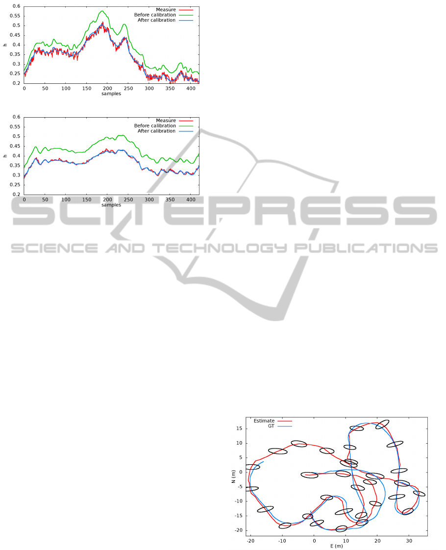
(a) X axis
(b) Y axis
Figure 5: A portion of the X-Y magnetometer readings
compared with predictions computed from q
W
O
(t), before
and after calibration for A and b.
tained by direct measurements on the vehicle (i.e.,
tape measure), or with default assignments such as
A = I and b = 0. The following covariance matrices
were assumed for the noise vectors η: Σ
GPS
= 0.69 I,
Σ
ACK
= diag(0.027,10, 100,10,100, 0.003), Σ
MAG
=
0.004 I and Σ
GY RO
= 0.003 I. We collected data
by means of an on-board PC, employing the system
clock to provide rough sensor reading timestamps.
The results of the calibration procedure were:
S
(O)
GPS
=
−0.52
1.14
8.30
q
O
S
IMU
=
0.997
0.003
−0.004
−0.079
A =
0.87 −0.02 −0.02
0.00 0.88 0.00
−0.02 −0.04 0.85
b =
−0.008
−0.007
−0.039
k
v
/L = 0.797 k
θ
= 1.043 k
γ
= 0.005
.
With the only exception of S
(O)
GPS
, all the estimated val-
ues, along with their covariance matrices, are consis-
tent with the direct measures. Moreover, the mag-
netometer calibration parameters A and b are able to
accommodate for the soft and iron distortion. Indeed,
given the estimated trajectory of the robot, from the
orientation at time t we can compute a prediction of
the magnetometer readings; in Figure 5 we compare
these predictions with the actual measurements before
and after the calibration of A and b.
Regarding S
(O)
GPS
, its estimate does not reflect the
direct measurements performed on the robot. Never-
theless, we note that the direct measurement of this
parameter is within the estimate confidence interval,
given its covariance matrix at the end of the Guass-
Newton optimization, which was:
Σ
S
(O)
GPS
=
0.118 0.001 −0.107
0.001 0.015 0.146
−0.107 0.146 8.049
.
Note that the z component is not observable given the
trajectory considered and this results in large variance
for the z component. We argue that the high uncer-
tainty and the lack of physical meaning of the esti-
mated S
(O)
GPS
is caused by limited timestamps accu-
racy, high noise, and limited frequency of the avail-
able data. To confirm this hypothesis, we repeated the
calibration employing the high accuracy RTK GPS
readings instead of the low cost Yuan10. This time the
result was S
(O)
RT K
= [0.71,−0.44,1.75], which is very
accurate with respect to direct measurements.
Finally we tested the on-line pose tracking system.
In the tracking benchmarks we consider windows of
60 poses. Again each new pose node is added ev-
ery time a new Ackermann odometry reading is avail-
able, i.e., every 0.05s. We compared the trajectory,
estimated from on-board sensors data, with the RTK
GPS measurements. The displacement of the refer-
ence RTK GPS with respect to the Yuan10 GPS sen-
sor used for tracking was carefully measured and can
be assumed to be S
(S
GPS
)
RT K
= [−0.29,−1.10,0.00]. In
Figure 6 we plot the position of the RTK GPS com-
puted from the estimate of O
(W )
and the ground truth.
It is possible to see that we are able to smoothly track
position and orientation of the robot despite the lim-
ited precision and sample rate of the Yuan10 GPS.
Figure 6: Ground truth RTK GPS readings and its position
S
(W )
RT K
computed from the estimate of O
(W )
, along with 3σ
uncertainties.
AFlexibleFrameworkforMobileRobotPoseEstimationandMulti-SensorSelf-Calibration
367

6 CONCLUSIONS AND FURTHER
WORK
In this work we have presented the ROAMFREE mo-
bile robot pose tracking and sensor self-calibration
framework along with experimental results about the
very first deployment of the framework to target the
Quadrivio ATV. ROAMFREE is being continuously
developed and our work focuses on the framework
structure, enriching the sensor library and improving
the sensor fusion techniques.
ROAMFREE is going to be extended to handle ac-
celeration measures. To do this, we plan to employ
Lie Groups operators to compute the finite difference
derivative of the pose nodes in the graph, consistently
working on the SE(3) manifold. This will also allow
us to interpolate the pose nodes in the graph assum-
ing constant acceleration and thus obtain virtual pose
nodes placed at the precise measurement timestamps.
We are also working on the extension of the cali-
bration suite to allow the estimation of latencies possi-
bly compromising measurement timestamps, and we
are considering to feedback the output of the on-line
tracking module to the logical sensors so that they can
take advantage of the accurate estimate of Γ
W
O
(t) to
update their internal state (i.e., update the tracked im-
age feature positions in a visual odometry system).
ACKNOWLEDGEMENTS
This work has been supported by the Italian Min-
istry of University and Research (MIUR) through the
PRIN 2009 grant “ROAMFREE: Robust Odometry
Applying Multi-sensor Fusion to Reduce Estimation
Errors”.
REFERENCES
Abe, M. and Manning, W. (2009). Vehicle handling dynam-
ics: theory and application. Butterworth-Heinemann.
Bascetta, L., Cucci, D., Magnani, G., Matteucci, M., Os-
mankovic, D., and Tahirovic, A. (2012). Towards
the implementation of a mpc-based planner on an au-
tonomous all-terrain vehicle. In In Proceedings of
Workshop on Robot Motion Planning: Online, Reac-
tive, and in Real-time (IEEE/RJS IROS 2012), pages
1–7.
Bascetta, L., Magnani, G., Rocco, P., and Zanchettin, A.
(2009). Design and implementation of the low-level
control system of an all-terrain mobile robot. In Ad-
vanced Robotics (ICAR), 2009 International Confer-
ence on, pages 1–6. IEEE.
Borenstein, J., Everett, H., and Feng, L. (1996). Where am
i? sensors and methods for mobile robot positioning.
University of Michigan, 119:120.
Bouvet, D. and Garcia, G. (2000). Improving the accu-
racy of dynamic localization systems using rtk gps by
identifying the gps latency. In Robotics and Automa-
tion (ICRA), 2000 IEEE International Conference on,
pages 2525–2530. IEEE.
Censi, A., Marchionni, L., and Oriolo, G. (2008). Simul-
taneous maximum-likelihood calibration of odome-
try and sensor parameters. In Robotics and Automa-
tion (ICRA), 2008 IEEE International Conference on,
pages 2098–2103. IEEE.
Chen, Z. (2003). Bayesian filtering: From kalman filters to
particle filters, and beyond. Statistics, 182(1):1–69.
Gill, P. E. and Murray, W. (1978). Algorithms for the so-
lution of the nonlinear least-squares problem. SIAM
Journal on Numerical Analysis, 15(5):977–992.
Harrison, A. and Newman, P. (2011). Ticsync: Know-
ing when things happened. In Robotics and Automa-
tion (ICRA), 2011 IEEE International Conference on,
pages 356–363. IEEE.
Hertzberg, C., Wagner, R., Frese, U., and Schr
¨
oDer, L.
(2013). Integrating generic sensor fusion algorithms
with sound state representations through encapsula-
tion of manifolds. Information Fusion, 14(1):57–77.
Horaud, R. and Dornaika, F. (1995). Hand-eye calibra-
tion. The international journal of robotics research,
14(3):195–210.
K
¨
ummerle, R., Grisetti, G., and Burgard, W. (2012). Simul-
taneous parameter calibration, localization, and map-
ping. Advanced Robotics, 26(17):2021–2041.
K
¨
ummerle, R., Grisetti, G., Strasdat, H., Konolige, K.,
and Burgard, W. (2011). g
2
o: A general framework
for graph optimization. In Robotics and Automa-
tion (ICRA), 2011 IEEE International Conference on,
pages 3607–3613. IEEE.
Martinelli, A., Tomatis, N., and Siegwart, R. (2007). Simul-
taneous localization and odometry self calibration for
mobile robot. Autonomous Robots, 22(1):75–85.
Quigley, M., Gerkey, B., Conley, K., Faust, J., Foote, T.,
Leibs, J., Berger, E., Wheeler, R., and Ng, A. (2009).
ROS: an open-source robot operating system. In ICRA
workshop on open source software, volume 3.
Vasconcelos, J., Elkaim, G., Silvestre, C., Oliveira, P.,
and Cardeira, B. (2011). Geometric approach to
strapdown magnetometer calibration in sensor frame.
Aerospace and Electronic Systems, IEEE Transac-
tions on, 47(2):1293–1306.
Weiss, S., Achtelik, M., Chli, M., and Siegwart, R. (2012).
Versatile distributed pose estimation and sensor self-
calibration for an autonomous mav. In Robotics and
Automation (ICRA), 2012 IEEE International Confer-
ence on, pages 31–38. IEEE.
ICINCO2013-10thInternationalConferenceonInformaticsinControl,AutomationandRobotics
368
