The Underwater Simulator UWSim
Benchmarking Capabilities on Autonomous Grasping
Javier P
´
erez, Jorge Sales, Mario Prats, Jos
´
e V. Mart
´
ı, David Fornas, Ra
´
ul Mar
´
ın and Pedro J. Sanz
IRS Lab, Jaume I University, Castellon, Spain
Keywords:
Benchmarking, Underwater Interventions, Datasets, Open Source Simulator.
Abstract:
Benchmarking is nowadays an issue on robotic research platforms, due to the fact that it is not easy to repro-
duce previous experiments and to know in detail in which real conditions other algorithms have been applied.
In the context of Underwater interventions with semi-autonomous robots the situation gets even more inter-
esting. Experiments performed by other researchers normally do not include the whole set of real conditions
such as visibility or even water currents data that would allow the best scientific procedure. Underwater
interventions and specially those performed on real sea scenarios are expensive, difficult to perform and repro-
duce. For this particular scenario, the use of an open platform simulation tool, with benchmarking capabilities
can provide an enormous help, as will be shown in the present paper. The Underwater Simulator UWSIM
(http://www.irs.uji.es/uwsim) has been shown to be a very useful tool for simulation, integration and bench-
marking, during the experiments performed in the context of the FP7 TRIDENT Project. In particular, in this
paper the use of the benchmarking capabilities of the UWSim platform for grasping autonomously an object
(airplane black box) from the sea floor in different water visibility and current conditions will be shown.
1 INTRODUCTION AND STATE
OF THE ART
Underwater manipulation using I-AUV (Autonomous
Underwater Vehivles for Intervention) makes it possi-
ble to design new applications such as the one studied
at the FP7 TRIDENT project, where a black box from
the sea bed was autonomously recovered. To accom-
plish this, the use of the UWSim (Underwater Sim-
ulator (Prats et al., 2012)) has been crucial, for both
testing and integration and also benchmarking.
There are previous simulators for underwater ap-
plications, which have mainly remained obsolete or
are being used for very specific purposes (Craighead
et al., 2007) (Matsebe et al., 2008). Moreover, the
majority of the examined simulators have not been
designed as open source, which makes difficult to im-
prove and enhance the capabilities of the simulator.
Moreover, there are other commercial simulators such
as ROVSim (Marine Simulation, ), DeepWorks (Fu-
gro General Robotics Ltd., ) or ROVolution (GRL.,
). However, they have been designed to train ROV
pilots, which is not the objective of the autonomous
grasping. In the following tables 1 and 2 a compar-
ative analysis between several underwater simulators
can be seen.
Table 1: Comparative Analysis on Underwater Simulators
(Part I)(Matsebe et al., 2008).
SUBSIM CADCON NEPTUNE MVS
Graphics 3D(openGl) 3D 3D(openGl) 3D
Type of Simulation Offline Online,HIL Online,HIL,HS Online,HIL,HS
Real Time NO YES YES YES
W
orld Modeling
YES
(Newton)
bath
ymetry
VRML YES
En
vironment Modeling
YES YES NO YES
Sensors YES YES YES YES
Multiple Vehicles NO YES YES YES
Distrib
uted System
NO YES YES YES
Supporting
Operating System
W
indows XP,98 /C,C++
IBM An
y
Type Open source Open source Open source Open source
Table 2: Comparative Analysis on Underwater Simulators
(Part II)(Matsebe et al., 2008).
DVECS IGW DeepWoks UWSim
Graphics 3D(openGl 3D 3D 3D(osg)
Type of Simulation Online,HIL,HS Online,HIL,HS Online,HIL Online,HIL,HS
Real Time YES YES YES YES
World Modeling YES YES YES YES(osgbullet)
Environment Modeling YES YES YES YES
Sensors YES YES YES YES
Multiple Vehicles YES NO NO YES
Distributed System YES YES NO YES
Supporting Operating System UNIX/C Windows Sistemas con ROS
Type Open source Open source Comercial Open source
On the other hand, the use of simulators to de-
fine specific benchmarks for underwater interventions
makes it possible to have a platform to better com-
pare, under the same conditions, the efficiency of two
different algorithms. Several definitions of bench-
marks have been proposed, but this work takes the one
explained at (Dillman, 2004) “adds numerical evalu-
ation of results (performance metrics) as a key ele-
ment. The main aspects are repeatability, indepen-
369
Pérez J., Sales J., Prats M., Martí J., Fornas D., Marín R. and Sanz P..
The Underwater Simulator UWSim - Benchmarking Capabilities on Autonomous Grasping.
DOI: 10.5220/0004484903690376
In Proceedings of the 10th International Conference on Informatics in Control, Automation and Robotics (ICINCO-2013), pages 369-376
ISBN: 978-989-8565-71-6
Copyright
c
2013 SCITEPRESS (Science and Technology Publications, Lda.)

dency, and unambiguity”. Some previous works on
benchmarking have been performed in other simula-
tors such as (Calisi et al., 2008) in stage, (Taylor et al.,
2008) in USARSim and (Michel and Rohrer, 2008) in
Webots. However, these works describe the develope-
ment of specific benchmarks instead of the design of a
platform for comparing algorithms. Moreover, in the
context of underwater robotics has been produces no
work of this kind before, to the best of our knowledge.
In this work a platform for the design of con-
figurable benchmarks is presented, created on the
UWSim simulator. In particular, two specific bench-
mark configurations are described. Firstly, the track-
ing algorithm is tested under different levels of vis-
ibity. After this, a specific benchmark to track and
control position over a black box in the sea floor is
presented, having different water currents as input.
The paper is organized as following. First of all
section 2 gives a summary of the main characteris-
tics of the benchmarking module. Sections 3 and 4
present the specific benchmarking examples, using
two experiments, the visibility test and the water cur-
rents respectively. Finally, section 6 concludes the ar-
ticle and provides a preview of further work.
2 DESIGN OF THE
BENCHMARKING MODULE
The benchmarking module has been implemented
in C++ and makes use of the UWSim simulator as
a library to carry out its mission. Like UWSim,
this application uses Robot Operating System (ROS)
(Quigley et al., 2009) for interfacing with external
software with which it can interact. ROS is a set of li-
braries that help software developers to create robotic
applications. It is a distributed system where differ-
ent nodes, which may be running on different com-
puters, are able to communicate by mainly publishing
and subscribing to “topics”. The ROS interface allows
the external program to be evaluated and can commu-
nicate both with the simulator (it can send commands
to carry out a task) and the benchmarking module (it
can send the results or data necessary to be evaluated).
For the development of the module, two important
objectives were taken into account. The first one is to
be transparent to the user, in other words, that it does
not require major modifications to the algorithm to be
evaluated. The other objective of the module is that
it must be adaptable to all kind of tasks, for exam-
ple, that it is possible to evaluate a vision system with
some disturbance tolerance for a particular scene.
To achieve these objectives, a Document Type Def-
BENCHMARK
MEASURES
TRIGGERSCENEUPDATER
CURRENT FOG NONE
TIME
OBJECT CAM
CENTERED
POSITION
ERROR
COLLISIONS DISTANCE
EUCLIDEAN
NORM
CONSTANT CORNERS CENTROID
POSITION
NOMOVE
MOVE
SERVICE
OFF
ON
TOPIC
N
ON, OFF
ON, OFF
Figure 1: Benchmark module structure.
inition (DTD) template has been defined, so that each
benchmark can be defined in a eXtensible Markup
Language (XML) file(Bray et al., 1997). A DTD is a
document that allows to establish the validity of XML
documents by defining its structure. In conclusion,
every time a user wants to create his own benchmark,
he must create an XML document that will define
which measures will be used and how them will be
evaluated. This will allow to create standard bench-
marks defined in a document to evaluate different as-
pects of underwater robotic algorithms, being able
to compare algorithms from different origins. Each
of these benchmarks will be associated with one or
more UWSim scene configuration files, being depen-
dent the results of the benchmark to the predefined
scene.
2.1 Module Structure
The implemented module has the structure shown in
Figure 1. It is a small structure with 4 main classes,
three of which have child classes thus being able to
add more functionality to the implemented module by
adding new derived classes as needed. This makes
the module easily extensible as it is only necessary
to implement a few prototype functions to extend the
usability of the module.
The “benchmark” class has different measures
that will be created as defined in the benchmark con-
figuration file. Each of these measures has a “trig-
ger” that sets the measure and another that stops it,
depending on the events specified in the configura-
tion. Besides this, the “benchmark” class has “scene-
Updaters” that modify the scene with each evalua-
tion of the algorithm. The operation of the module is
simple: for each configuration of the scene indicated
by the chosen “SceneUpdater”, the measures are cre-
ated and they are activated or deactivated according
to the “triggers”. These measures evaluate the algo-
rithm with a score that is stored for each iteration of
the “SceneUpdater”. Finally, when all the scene con-
figurations have been evaluated, the benchmark ends
and returns an output file with the results. These re-
sults are disaggregated for each configuration of the
ICINCO2013-10thInternationalConferenceonInformaticsinControl,AutomationandRobotics
370
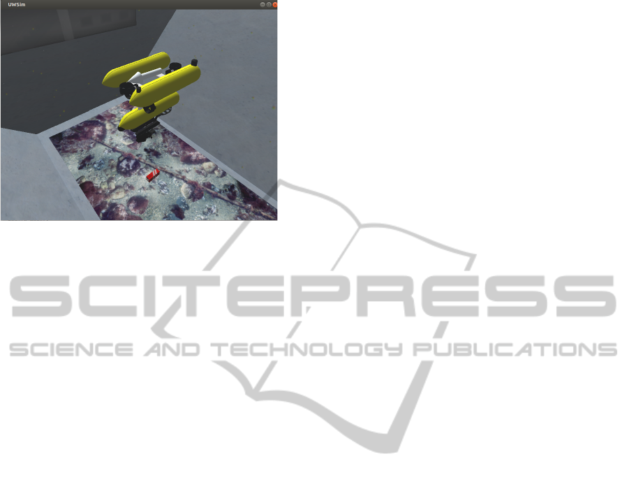
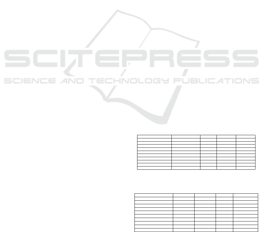
Figure 2: Underwater current benchmark scene.
scene, containing both individual measures and the
overall score of them, which is a function defined in
the XML file.
Furthermore measures can be logged as time
passes in order to see it’s evolution through the ex-
periment. These feature allows to analyze the per-
formance of the algorithm to be evaluated with the
benchmarking platform and not only the final results.
2.2 Module Features
The features of the benchmarking module are defined
by the “triggers”, “sceneUpdaters” and measures im-
plemented, and can be freely configured to suit any
situation. Therefore, below is the description of the
options that are already implemented. These are the
current measures already implemented.
• Time: This measure returns the elapsed seconds
between the “start” and “stop” triggers created for
this measure.
• Collisions: This class uses osgBullet(Coumans, )
to measure the collision of a specified object or
vehicle. For this purpose, it extracts the maxi-
mum and average collision speeds and percentage
of time in contact with other objects. Note that the
collision velocities are measured from the veloc-
ity of the two objects that collide in the direction
of the vector that connects them.
• PositionError: This measure returns the position
error of an object or vehicle with respect to a po-
sition defined by the benchmark. It can be used to
measure whether a vehicle has released an object
in a correct position. For example, in the case of
a robot that performs pick and place of submarine
pipelines, it can measure its performance accord-
ing to the position of the pipes at the end of the
intervention.
• Distance: In this case, the distance (in meters) that
a vehicle has traveled is measured. As an exam-
ple, is the one that will be preferred, the algorithm
that makes the vehicle to move fewer meters dur-
ing an intervention.
• EuclideanNorm: This measure calculates the Eu-
clidean norm between two vectors. The first of
these two vectors can be specified in advance
(ground truth) or calculated automatically to find
the centroid or the corners of an object in a virtual
camera. The second one is received from a ROS
“topic”. This measure is used when the result of
the algorithm to be evaluated cannot be directly
obtained into the simulator, such as the result of a
tracker.
• ObjectCamCentered: With this label, the position
error of an object with respect to the center of the
camera is calculated.
These are the measures that have been imple-
mented until now, but there are more being designed,
to be able to model a large diversity of benchmarks.
Some of the measures that can be implemented are
related to battery consumption or control of the ve-
hicle. All these measures provide many different op-
tions when evaluating an algorithm, however it is nec-
essary to control them when they are turned on and
off. This functionality is covered by the “triggers”.
Below is the description of the ones already imple-
mented in the UWSim module.
• TopicTrigger: Allows starting or stopping a mea-
surement when any information is received on a
ROS “topic”.
• AlwaysOnTrigger: Indicates that the measure
must be active all the time.
• AlwaysOffTrigger: Let measures not be disabled
in the case of any event.
• ServiceTrigger: Version that uses a service rather
than a “TopicTrigger” topic.
• MoveTrigger: This trigger is activated when the
object indicated in its creation has moved more
than a threshold defined in a global variable.
• NoMoveTrigger: As its name indicates, in this
case the trigger is activated when a vehicle or ob-
ject stops moving.
• PositionTrigger: This trigger is activated when a
vehicle or object reaches a specified position.
Finally, the “sceneUpdaters” define how the
scenes changes as time passes to evaluate the algo-
rithm in different situations. At the moment there are
only three, although it is planned to add more when
water physics is ready on UWSim or otherwise as
TheUnderwaterSimulatorUWSim-BenchmarkingCapabilitiesonAutonomousGrasping
371
needed. The “sceneUpdaters” implemented so far are
the following:
• NullSceneUpdater: This updater does not update
the scene. That is, the benchmark will run only
once with the existing scene conditions.
• SceneFogUpdater: It updates the scene from a
minimum underwater fog level to a maximum, by
adding the specified amount. For each fog level,
the measures are calculated and the benchmark
score is stored.
• CurrentForceUpdater: In this case, the force of the
current is progressively increased. However the
rest of the current options (direction, variability,
randomness) are unchanged. These updater can
be easily modified to accept custom currents.
3 USE CASE: VISIBILITY
This tool allows benchmarking with many config-
urable options. Algorithms can be tested to their lim-
its, to know under which conditions can they work,
and which results can be obtained with them. This
way resources can be optimized to provide the best
results in each situation.
Below is an example of benchmarking done with
UWSim. In this case, the goal is to evaluate how the
underwater fog affects a visual ESM tracking algo-
rithm (Malis, 2004). Firstly a scenario with suitable
conditions to do tracking is created. This scenario in-
cludes the representation of the pool at the Underwa-
ter Robotics Research Center (CIRS), Girona, Spain,
with the Girona500 vehicle and the ARM5E arm. The
scenario has a virtual camera located above a black
box. It is only possible to access the “topics” of the
virtual camera, so the vehicle cannot move thus avoid-
ing errors when evaluating the vision system. The
scene can be seen in Figure 3. In the scene, the ve-
hicle appears in the pool and on the lower left corner
of the scene, a virtual camera can be seen pointing at
the black box.
In addition to the scene, a benchmark configu-
ration file has been designed. It includes measure
definitions used to evaluate the performance of the
tracking and all that is needed to evaluate the track-
ing software. Since the tracking algorithm returns
the position of a four-corner object, an “euclidean-
Norm” measure is used, which measures the distance
between the position returned by the tracking soft-
ware and the real position on the simulator.
This distance is divided in two parts to get more
information. On one hand, the distance between the
Figure 3: Vision benchmark scene.
Figure 4: Tracking algorithm screenshots for decreasing
visibility in the benchmark.
actual corners with the ones that the tracking algo-
rithm returns. On the other hand, the real distance
from the centroid of the simulated object to the one
calculated through vision. For the final result, these
two measurements are added so that the lower the re-
sult, the smaller the object recognition error is. In
addition to these measurements, the scene updater
“sceneFogUpdater” is configured varying the under-
water scene visibility through time.
Finally, some triggers have been set up to make the
evaluation task easier. For the beginning of the bench-
mark, benchmark module will wait for a service call
made by the tracking algorithm, and it will end when
there are no more “sceneFogUpdater” iterations. The
measurements will always be active, as it is taken as
valid the last one received by the ROS “topic” that the
vision system sends.
Once the simulator and the benchmark are con-
figured, a service call must be added in the tracking
algorithm when it starts, and the estimated position of
the box must be sent. As shown on figure 4 the track-
ing algorithm is able to find the black box while the
fog is increasing in the benchmark, until finally it is
completely lost when the visibility is very low.
Once the benchmark is complete, the module
stores the results in a file. These results are stored
in a text file in table format. This file can be pro-
cessed later with any statistical or graphical tool. For
this case study the results can be seen on Figure 5.
ICINCO2013-10thInternationalConferenceonInformaticsinControl,AutomationandRobotics
372
0
20
40
60
80
100
120
0 0.2 0.4 0.6 0.8 1 1.2
Benchmark score (pixels error)
Fog value
Benchmark for tracking with different fog values
Figure 5: Visibility benchmark results.
0
2
4
6
8
10
12
14
16
0 0.2 0.4 0.6 0.8 1 1.2
Benchmark score (pixels error)
Fog value
Benchmark for tracking with different fog values (only centroid)
Figure 6: Visibility benchmark results for the centroid lo-
calization.
It can be observed how the tracking software error is
very small throughout the experiment, less than 5 er-
ror pixels between corners and the centroid. For a fog
level of 1.1, the error increases and the tracking algo-
rithm aborts when it completely loses the target.
Besides this, graphs can be drawn for each mea-
surement separately. Figures 6 and 7 show respec-
tively the error in the location of the centroid and the
corners of the box. As can be seen, the error in the
centroid is stable with some minor noise for values
smaller than a pixel, while the error in the corners in-
creases with increasing level of fog.
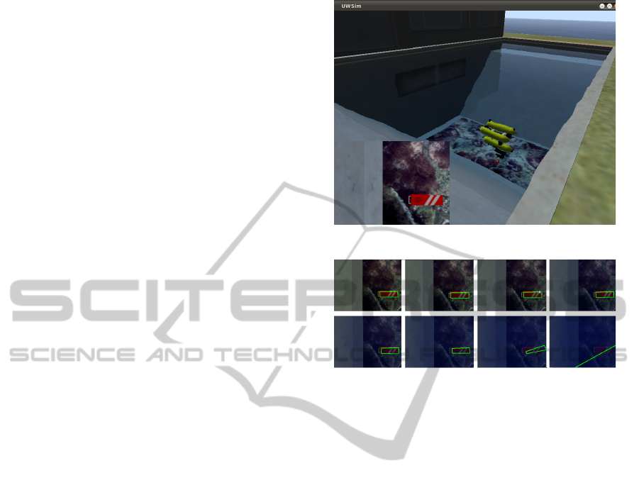
According to the results provided, the vision sys-
tem is reliable for fog levels below 1.1. Figures 8
and 9 show a comparison between this levels of fog
on UWSim simulator screenshots. The fog level is a
value ranging from 0 to infinity and defines the vis-
ibility in the water depending on the distance. Visi-
bility is a value between 0 and 1 where 0 represents a
perfect visibility of the object and 1 represents no vis-
ibility at all. The visibility depends therefore on the
water fog level and on the distance to the object, as it
is represented by the following formula:
visibility = 1 − e
−( f og f actor∗distance)
2
(1)
0
10
20
30
40
50
60
70
80
90
100
0 0.2 0.4 0.6 0.8 1 1.2
Benchmark score (pixels error)
Fog value
Benchmark for tracking with different fog values (only corners)
Figure 7: Visibility benchmark results for corners localiza-
tion.
Figure 8: Comparison between fog levels 0 and 1.1 in the
simulator.
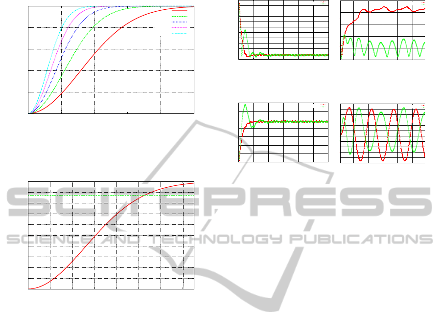
In Figure 10 different values have been used to
plot the relationship between visibility and the dis-
tance to the object. As can be seen, visibility drasti-
cally worsens with relatively small values of fog when
the distance to the object increases. Under a 1.05
value of fog (represented with purple line, which was
the operating limit of the tracking software), there is
virtually no visibility for a distance greater than 2 me-
ters.
In Figure 11 the distance to the object has been set
to 1.36 meters, which is actually the distance between
the camera and the black box in the benchmark, and
it represents the visibility with respect to the fog fac-
tor. The value of visibility for a fog factor of 1.1 is
depicted with a horizontal line. Thus the tracking al-
gorithm is able to find an object when the degree of
visibility is below 0.86.
Figure 9: Comparison between fog levels 0 and 1.1 in the
simulator’s camera.
TheUnderwaterSimulatorUWSim-BenchmarkingCapabilitiesonAutonomousGrasping
373
0
0.2
0.4
0.6
0.8
1
0 1 2 3 4 5
Distance to obstacle (meters)
fog factor
Visibility distance depending on fog factor
0.45
0.65
0.85
1.05
1.25
Figure 10: Visibility and distance relation for different fog
levels.
0
0.1
0.2
0.3
0.4
0.5
0.6
0.7
0.8
0.9
1
0 0.2 0.4 0.6 0.8 1 1.2 1.4
visibility
fog factor
Visibility fog factor at fixed distance 1.36
Figure 11: Visibility and fog factor relation for a fixed dis-
tance of 1.36 metres.
4 USE CASE: UNDERWATER
CURRENTS
Besides the previous example, this platform has been
used to measure the results of two positioning con-
trol algorithms for an underwater vehicle over a tar-
get. The goal is to maintain the vehicle over the tar-
geted black box despite the influence of currents, with
just a camera as sensor. The benchmarking module is
able to contrast and compare the results of two simple
controllers designed for this purpose.
The scenario is almost the same as the one used
in the visibility example. But now an increasing sinu-
soidal current is pushing the vehicle as shown on fig-
ure 2 represented by an arrow. Users can define more
realistic currents creating a function that returns force
and direction in every time step for a specific vehicle.
Besides this, velocity topics have been configured to
control the vehicle’s positioning.
For the benchmark configuration an “Object Cen-
tered On Cam” measure has been included on the
benchmark configuration in order to evaluate the con-
0
5
10
15
20
25
30
35
40
45
50
55
0 20 40 60 80 100 120
Distance to objective (pixels)
Time (seconds)
Distance to objective vs time
P controller
PI controller
0
50
100
150
200
250
2300 2320 2340 2360 2380 2400
Distance to objective (pixels)
Time (seconds)
Distance to objective vs time
P controller
PI controller
Figure 12: Distance to objective(left no current, right 0.2
m/s current).
-25
-20
-15
-10
-5
0
5
10
0 20 40 60 80 100 120
Error (pixels)
Time (seconds)
Positioning error vs time
P controller
PI controller
-120
-100
-80
-60
-40
-20
0
20
40
60
80
100
2300 2320 2340 2360 2380 2400
Error (pixels)
Time (seconds)
Positioning error vs time
P controller
PI controller
Figure 13: Current control positioning error on X axis(left
no current, right 0.2 m/s current).
troller. This measure will be logged in a different
result file with two components according to camera
axis errors. Tracking error is still measured in order
to see if the positioning controller affects it.
The designed controllers are: a P controller that
produces an output proportional to the positioning
error measured by the tracker. And a PI controller
which adds an integral term to the proportional out-
put. Much better controllers can be designed for this
experiment, but the aim of it is to demonstrate the ca-
pabilities of the developed benchmark platform eval-
uating controllers, instead of designing a good con-
troller.
In contrast to the previous use case, in this exper-
iment final results are not so important. The position-
ing error evolution through time is much more use-
ful. As shown on figure 12 P (red) and PI (green)
controllers try to reduce the distance error in two dif-
ferent environments. In the left-hand graph there is
no current pushing the vehicle and in the right-hand
graph a great current pushes it. This is only a small
piece of the whole experiment where different current
forces are used to measure the perfomance of both
controllers.
As expected the PI controller works better, but it
can’t control the sinusoidal perturbations completely
(maybe a better design of the PI controller will make
it, but this is not the aim of the work). These kinds of
results can help to improve the design of controllers,
but the benchmarking platform can give information
split in camera-axis to make an easier analysis of the
process. The figures 13 14, show this feature repre-
senting the X and Y error respectively. In those pic-
tures the sinusoidal perturbations applied in the X-
axis of the current are being transferred to the out-
put and therefore a different controller should be de-
ICINCO2013-10thInternationalConferenceonInformaticsinControl,AutomationandRobotics
374
-30
-20
-10
0
10
20
30
40
50
0 20 40 60 80 100 120
Error (pixels)
Time (seconds)
Positioning error vs time
P controller
PI controller
-250
-200
-150
-100
-50
0
50
100
2300 2320 2340 2360 2380 2400
Error (pixels)
Time (seconds)
Positioning error vs time
P controller
PI controller
Figure 14: Current control positioning error on Y axis(left
no current, right 0.2 m/s current).
0
5
10
15
20
25
30
35
40
0 0.02 0.04 0.06 0.08 0.1 0.12 0.14 0.16 0.18 0.2
Centroid error (pixels)
Current force (meters/seconds)
Current vs tracking centroid
Figure 15: Tracker error on underwater current benchmark
for each controller.
signed. On the Y-axis PI controller is much better
than P, driving the error to zero in different conditions
while P error depends on the force of the current.
Finally on figure 15 the tracker error for each con-
troller (P red, PI green) is shown. It’s quite interest-
ing to see that the PI controller helps in some way the
tracker making smoother movements so the objective
is not lost. Although the tracker on the P controller
works fine, it has a slightly bigger error than PI caused
by drastic moves.
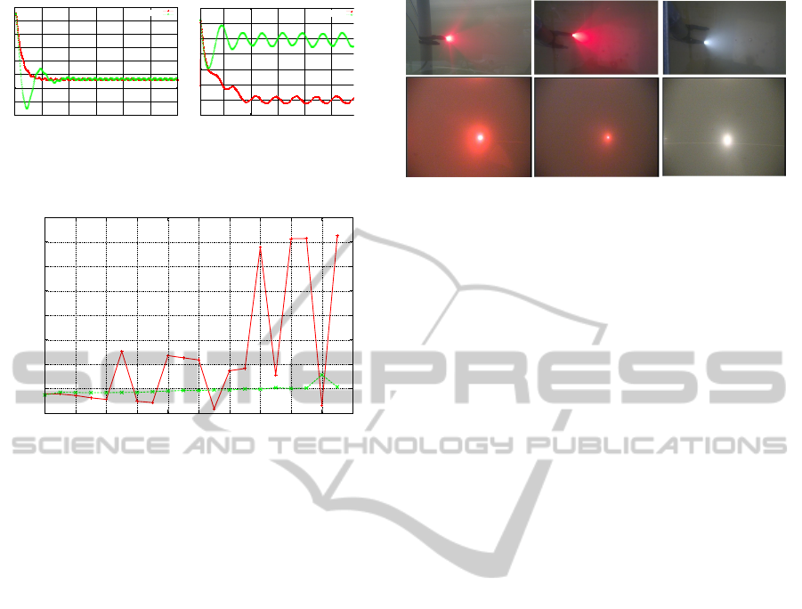
5 VALIDATION IN A REAL
LABORATORY SCENARIO
In the subsea context, the quality of the images cap-
tured by the camera mounted on the autonomous
robots, can be strongly affected by the degree of the
water turbidity. In unfavorable circumstances, the dis-
tance at which this device is usable (ie, the range of
visibility) is the required parameter in order to know
to make a proper use of it. On the other hand, when
the image captured by the camera does not contain
objects near the robot, it is not possible to determine
whether the absence is due to the fact that there are re-
ally no objects near the vehicle or that water turbidity
prevents their vision.
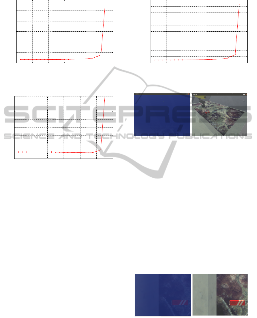
To have a metric to determine the maximum dis-
tance at which the camera is effective at each instant,
Figure 16: Underwater visibility experimental results on in-
creasing water turbidity.
a calibration experiment has been developed. Two
high intensity LEDs (one red and one white), placed
at a fixed distance from the camera, have been used
as shown on figure 16. To reach this fixed distance
the diodes can be placed in the submarine’s robotic
arm and then it can be moved properly until the LEDs
reach the calibration location. On the other hand, a
calibration image that is positioned at a distance of 1
meter from the camera and is lightened by the built-it
autonomous robot focus has been made.
To muddy the water, a special dye for decorative
paintings has been used: a powder containing parti-
cles of different sizes. Thus, the water in the container
in which the experiment has been developed, progres-
sively blurred without having absolute measurements
of turbidity. For each concentration of dye, in the ab-
sence of ambient light,the vehicle’s built-in light has
been activated to illuminate the test image, and then a
screenshot of the captured image has been taken. Af-
ter that, with the lights turned off, the red and white
LEDs have been alternatively activated taking screen-
shot of each of them.
The three images form the calibration of the de-
gree of visibility of the focus-camera set for this par-
ticular conditions of turbidity. Thus, the aspect of
each of the LEDs makes it possible to determine the
degree of visibility at 1 meter of distance and this can
be used as a starting point for an estimation of the
maximum distance that will have some degree of vis-
ibility.
6 CONCLUSIONS AND FURTHER
WORK
In this paper the benchmarking characteristics of the
UWSim (Underwater Simulator) software have been
presented, which permits the design of specific ex-
periments on autonomous underwater interventions.
More specifically, the simulator allows the integra-
tion, in a unique platform, of the data acquired from
the sensors in a real submarine intervention and de-
TheUnderwaterSimulatorUWSim-BenchmarkingCapabilitiesonAutonomousGrasping
375
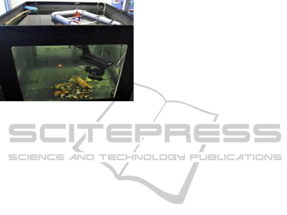
Figure 17: Underwater platform with ARM5E robotic arm
used perform water current tests.
fine a dataset, in order to allow further experiments to
work on the same scenario, permitting a better under-
standing of the results provided by previous experi-
ments. Moreover, the paper focused on the effect of
both, limited visibility conditions and water currents,
on the tracking algorithm. Detailed benchmarks have
been designed to take into account these specific con-
ditions, and extract which are the scenarios where the
autonomous intervention algorithms are able to work
properly.
To better validate the results, similar real exper-
iments in lab conditions have been presented. For
example, to validate the simulated results on the
real platform a water tank is being used to repro-
duce the simulated conditions as shown on figure
17, and high luminosity LEDs are used for calibra-
tion purposes. Similarly, the current effects are val-
idated using a robot mobile platform that is able
to introduce disturbances on the robot movements,
simulating a more realistic scenario. The UWSim
software is provided to the public as open source
http://www.irs.uji.es/uwsim, and it is included as a
module within the ROS (Robotic Operating System)
platform http://ros.org/wiki/UWSim.
Further work will focus on the design of hardware
in the loop benchmarking, providing a better corre-
spondence between the simulated and the real results.
ACKNOWLEDGEMENTS
This research was partly supported by Spanish Min-
istry of Research and Innovation DPI2011-27977-
C03 (TRITON Project), by the European Commis-
sion Seventh Framework Programme FP7/2007-2013
under Grant agreement 248497 (TRIDENT Project),
by Foundation Caixa Castell-Bancaixa PI.1B2011-
17, and by Generalitat Valenciana ACOMP/2012/252.
REFERENCES
Bray, T., Paoli, J., Sperberg-McQueen, C. M., Maler, E.,
and Yergeau, F. (1997). Extensible markup language
(xml). World Wide Web Journal, 2(4):27–66.
Calisi, D., Iocchi, L., and Nardi, D. (2008). A unified
benchmark framework for autonomous mobile robots
and vehicles motion algorithms (movema bench-
marks). In Workshop on experimental methodology
and benchmarking in robotics research (RSS 2008).
Coumans, E. Bullet physics library (2009). Available on-
line: http://bulletphysics.org/.
Craighead, J., Murphy, R., Burke, J., and Goldiez, B.
(2007). A survey of commercial open source un-
manned vehicle simulators. In Robotics and Automa-
tion, 2007 IEEE International Conference on, pages
852 –857.
Dillman, R. (2004). Ka 1.10 benchmarks for robotics re-
search. Technical report, Citeseer.
Fugro General Robotics Ltd. Deepworks. Available online:
http://www.fugrogrl.com/software/.
GRL. Rovolution.
Malis, E. (2004). Improving vision-based control using
efficient second-order minimization techniques. In
Robotics and Automation, 2004. Proceedings. ICRA
’04. 2004 IEEE International Conference on, vol-
ume 2, pages 1843 – 1848 Vol.2.
Marine Simulation. ROVsim. Available online: http://
marinesimulation.com.
Matsebe, O., Kumile, C., and Tlale, N. (2008). A review
of virtual simulators for autonomous underwater ve-
hicles (auvs). NGCUV, Killaloe, Ireland.
Michel, O. and Rohrer, F. (2008). The rat’s life benchmark:
competing cognitive robots. In Proceedings of the 8th
Workshop on Performance Metrics for Intelligent Sys-
tems, PerMIS’08, pages 43–49, New York, NY, USA.
ACM.
Prats, M., P
´
erez, J., Fern
´
andez, J., and Sanz, P. (2012).
An open source tool for simulation and supervision
of underwater intervention missions. In Intelligent
Robots and Systems (IROS), 2012 IEEE/RSJ Interna-
tional Conference on, pages 2577 –2582. IEEE.
Quigley, M., Gerkey, B., Conley, K., Faust, J., Foote, T.,
Leibs, J., Berger, E., Wheeler, R., and Ng, A. (2009).
Ros: an open-source robot operating system. In ICRA
workshop on open source software, volume 3.
Taylor, B., Balakirsky, S., Messina, E., and Quinn, R.
(2008). Analysis and benchmarking of a whegs robot
in usarsim. In Intelligent Robots and Systems, 2008.
IROS 2008. IEEE/RSJ International Conference on,
pages 3896 –3901.
ICINCO2013-10thInternationalConferenceonInformaticsinControl,AutomationandRobotics
376
