
Topological Map Building and Path Estimation Using Global-appearance
Image Descriptors
F. Amor
´
os
1
, L. Pay
´
a
1
, O. Reinoso
1
, W. Mayol-Cuevas
2
and A. Calway
2
1
Dep. de Ingenier
´
ıa de Sistemas y Autom
´
atica, Miguel Hern
´
andez University,
Avda. de la Universidad, s/n. 03202, Elche (Alicante), Spain
2
Department of Computer Science, University of Bristol,
Woodland Road BS8 1UB, Bristol, United Kingdom
Keywords:
Map Building, Topological Graph, Image Scale Comparison, Global-appearance Descriptor.
Abstract:
Visual-based navigation has been a source of numerous researches in the field of mobile robotics. In this paper
we present a topological map building and localization algorithm using wide-angle scenes. Global-appearance
descriptors are used in order to optimally represent the visual information. First, we build a topological graph
that represents the navigation environment. Each node of the graph is a different position within the area, and it
is composed of a collection of images that covers the complete field of view. We use the information provided
by a camera that is mounted on the mobile robot when it travels along some routes between the nodes in the
graph. With this aim, we estimate the relative position of each node using the visual information stored. Once
the map is built, we propose a localization system that is able to estimate the location of the mobile not only
in the nodes but also on intermediate positions using the visual information. The approach has been evaluated
and shows good performance in real indoor scenarios under realistic illumination conditions.
1 INTRODUCTION
The autonomous navigation of a mobile agent in a
certain environment usually requires an inner repre-
sentation of the area, i.e. a map, that the robot will
interpret in order to estimate its current position using
the information provided by the sensors it is equipped
with. Among all the possible sensors a robot can
use to achieve that purpose, in this paper we focus
on a visual system, since it constitutes a rich source
of information and the sensors are relatively inexpen-
sive. Specifically, in this work we use a fish-eye sin-
gle camera, which provides wide angle images of the
environment.
A key task in vision based navigation is match-
ing. Through the matching of the current robot sensor
view with previous information that constitutes the
robot’s map, it is possible to carry out its localization.
Usually, this is achieved by extracting some features
from the image in order to create a useful descriptor
of the scene with a relative low dimension to make it
useful in real time operation. In this task, two main
categories can be found: feature based and global-
appearance based descriptors. The first approach is
based on the extraction of significant points or regions
from the scene. Popular examples include SIFT fea-
tures (Lowe, 2004) or SURF (Murillo et al., 2007).
On the other hand, global-appearance descriptors try
to describe the scene as a whole, without the extrac-
tion of local features or regions. For example, (Krose
et al., 2007) make use of PCA (Principal Component
Analysis) to image processing, and (Menegatti et al.,
2004) take profit of the properties of the Discrete
Fourier Transform (DFT) of panoramic images in or-
der to build a descriptor that is invariant to the robot’s
orientation. Regarding the map representation of the
environment, the existing research can be categorized
in two main approaches: metric and topological. Met-
ric maps include information such as distances respect
to a predefined coordinate system. In this sense, we
can find examples as (Moravec and Elfes, 1985), that
presents a system based on a sonar sensor applied
to robot navigation, and (Gil et al., 2010), that de-
scribes an approach to solve the SLAM problem us-
ing a team of robots with a map represented by the
three-dimensional position of visual landmarks. In
contrast, topological techniques represent the envi-
ronment through a graph-based representation. The
nodes correspond to a feature or zone of the environ-
ment, whereas the edges represent the connectivity
385
Amoros F., Paya L., Reinoso O., Mayol-Cuevas W. and Calway A..
Topological Map Building and Path Estimation Using Global-appearance Image Descriptors.
DOI: 10.5220/0004485203850392
In Proceedings of the 10th International Conference on Informatics in Control, Automation and Robotics (ICINCO-2013), pages 385-392
ISBN: 978-989-8565-71-6
Copyright
c
2013 SCITEPRESS (Science and Technology Publications, Lda.)

between the nodes. In (Gaspar et al., 2000) a visual-
based navigation system is presented using an omni-
directional camera and a topological map as a rep-
resentation in structured indoor office environments.
(Frizera et al., 1998) describe a similar system which
is developed using a single camera.
In (Cummins and Newman, 2009), a SLAM sys-
tem called FAB-MAP is presented. The description of
the scenes is based on landmark extraction. Specifi-
cally, they use SURF features, and their experimental
dataset is a very large scale collection of outdoor om-
nidirectional images. Our aim is to develop a similar
system but using a wide-angle camera (which is more
economical than catadioptric or spherical vision cam-
era systems). Another difference is the kind of infor-
mation we use to describe the images, since we use
global-appearance descriptors.
The first step in our work consists in building a
map of the environment. We use a graph representa-
tion. In this representation, each node is composed of
8 wide-angle images that cover the complete field of
view from a position in the environment to map, and
the edges represent the connectivity between nodes to
estim.
In order to estimate the topological relationships
between nodes, we use the information extracted from
a set of images captured along some routes which pass
through the previously captured nodes. As a contribu-
tion of this work, we apply a multi-scale analysis of
the route and node’s images in order to increase the
similarity between them when we move away form
a node. From this analysis, we obtain both an in-
crease of correct matching of route images in the map
database, and also a measurement of the relative po-
sition of the compared scenes.
Once the map is built, as a second step we have
designed a path estimation algorithm that also takes
profit of that scale analysis to extrapolate the position
of the route scenes not only in the nodes but also in
intermediate points. The algorithm, which is also a
contribution of this work, introduces a weight func-
tion in order to improve the localization precision.
The remainder of the paper is structured as fol-
lows. Section 2 introduces the features of the
dataset used in the experimental part, and the global-
appearance descriptor selected in order to represent
the scenes. Section 3 presents the algorithm devel-
oped to build the topological map. In Section 4 we
explain the system that builds the representation of
route paths, and experimental results. Finally, in Sec-
tion 5 we summarize the main ideas obtained in this
work.
TERMINOLOGY: We use the term node to refer
to a collection of eight images captured from the same
position on the ground plane every 45
◦
, covering the
complete field of view around that position. We de-
note the collection of images of the nodes as map’s
images or database’s images. The graph that rep-
resents the topological layout of the nodes is named
map. The process of finding the topological connec-
tion between nodes and their relative position is the
map building. We call the relative position between
nodes topological distance. When we write image
distance we refer to the Euclidean distance between
the descriptors of two images. The topological dis-
tance between two images is denoted as l, and the
topological distance between nodes as c.
2 DATA SET AND DESCRIPTOR
FEATURES
In this section, we present the features of the images’
data set, and the global-appearance technique we use
in order to create a descriptor of the scenes.
The images are captured using a fisheye lens cam-
era. We choose this kind of lens due to its wide-angle
view. Specifically, the model used is the Hero2 of Go-
Pro (Woodman Labs, 2013). The angle of view of the
images is 127
◦
. Due to the fisheye lens, the scenes
present a distortion that makes it impossible to ob-
tain useful information from the images using global-
appearance descriptors, since they are based on the
spatial distribution and disposition of the elements in
the scene, and the distortion makes the elements to ap-
pear altered. For that reason, we use the Matlab Tool-
box OCamCalib in order to calibrating the camera
and computing the undistorted scenes from the origi-
nal images (Scaramuzza et al., 2006). In the reminder
of the paper, the term image refers to the undistorted
transform of the original scenes.
Since the aim of this work is to solve the problem
of place recognition using the global-appearance of
images, it is necessary to use descriptors that concen-
trate the visual information of the image as a whole,
being also interesting the robustness against illumi-
nation changes and the capacity of dealing with little
changes in the orientation of the scenes. Some works,
as (Paya et al., 2009), have compared the perfor-
mance of some global-appearance descriptors. Taking
them into account, we have decided to choose Gist-
Gabor descriptor (Torralba, 2003), (Oliva and Tor-
ralba, 2001) as it presents a good performance in im-
age retrieval when working with real indoor images.
It also shows a reasonable computational cost. With
an image’s size of 64x32 pixels, the algorithm spent
0.0442 seconds to compute the descriptor using Mat-
lab R2009b running over a 2.8 GHz Quad-Core Intel
ICINCO2013-10thInternationalConferenceonInformaticsinControl,AutomationandRobotics
386
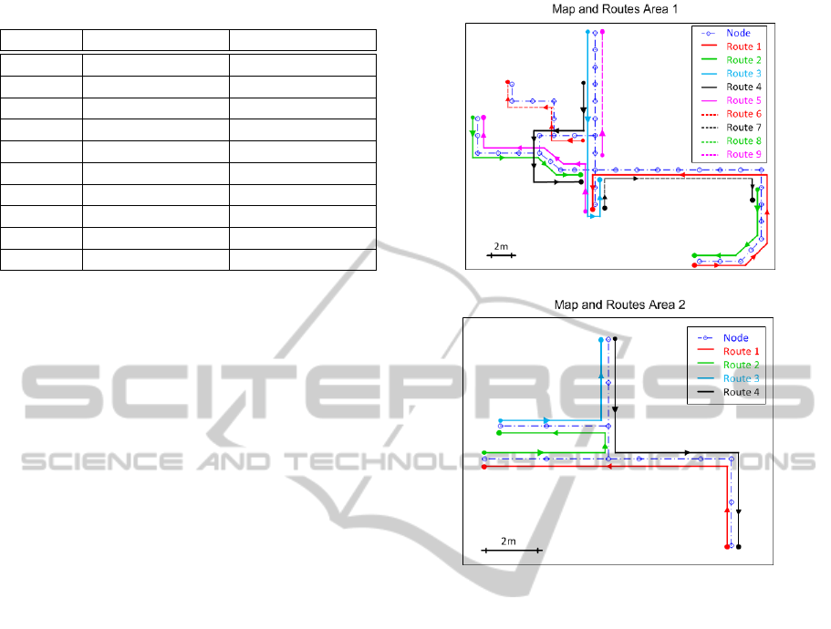
Table 1: Number of Images per Area
# Images Area 1 # Images Area 2
Nodes 352 52
Route 1 110 100
Route 2 50 72
Route 3 67 66
Route 4 58 125
Route 5 62 -
Route 6 46 -
Route 7 69 -
Route 8 67 -
Route 9 40 -
Xeon processor, requiring 4,096 bytes of memory per
image.
The dataset is divided in two different areas. The
Area 1 is composed of 44 nodes, whereas Area 2 has
13 nodes. The nodes are taken every 2 meters as a
rule, but in places where an important change of ap-
pearance in the area is produced, i.e. crossing a door,
we capture a new node independently of the distance.
For that reason, the distance may be lower. As stated
above, each node has 8 images captured every 45
◦
approximately regarding the floor plane, covering the
complete field of view.
We have also captured images along routes in both
areas. The information of those routes is used first
in order to find the topological relationships between
nodes and build the graph representation in the map
building task, and next to carry out the path estima-
tion of those routes in the localization experiments.
Regarding the routes, the images are taken every 0.5
meters in Area 1, and every 0.2 meters in Area 2. In
changes of direction, we increase the frequency of im-
ages captured. We take a minimum of four images per
position when a change of orientation is produced. In
Area 2, that frequency increases with a minimum of
6 images per position. In Fig. 1 we can see the dis-
tribution of the nodes and the routes in a synthetic
representation.
3 MAP BUILDING
In this section we describe the algorithm we have de-
veloped in order to create the robot’s inner represen-
tation of the environment. Since we propose a topo-
logical representation, the map building process relies
on finding the adjacency relations and relative dispo-
sition of the nodes to create the map. For that pur-
pose, we use the route images. So then, the map is
built as a graph were the nodes represent a location
of the environment, whereas the edges provides infor-
(a)
(b)
Figure 1: Synthetic distribution of nodes and routes for (a)
Area 1 and (b) Area 2.
mation about the topological distance and direction of
adjacent nodes. We have no previous information nei-
ther about the order of the nodes nor its disposition in
the world. However, we know in which order the 8
images of each node were captured. The node’s im-
ages make up a retrieval database. The system uses
the images of the route to arrange and find the spatial
relations between nodes by matching its images with
the map’s images. Since the route images are ordered,
we add information to the map’s graph incrementally
through the retrieval of the node’s images using the
route scenes.
In this process, we make use of some artificial
zooms of the images to increment the likelihood of
retrieving the correct nearest node’s image given a
route image. In Fig. 2 we can see a representation
of the disposition of the route’s images regarding the
nodes, and examples of the scenes. Figure 2(b) is an
image of the route, Fig. 2(a) is the closest node’s
image, and Fig. 2(a’) represents a zoom in of the
node’s image. Comparing the route image with both
the original node’s image and its zooms in, we can
realize that the appearance is more similar with the
zoomed scene. This is especially interesting for find-
TopologicalMapBuildingandPathEstimationUsingGlobal-appearanceImageDescriptors
387

ing the correspondence of images located halfway of
two nodes, since the similarity in that positions signif-
icantly decreases regarding the nearest nodes. Using
the zooms we increase the probability of a correct re-
trieval.
In our algorithm, we use zooms in of both the
node’s images and the route’s images. Given a
route image, the algorithm compares several scales of
this image with different scale representations of the
node’s images. After these comparisons, we select
the experiment with the minimum image distance. s
n
and s
r
represent the specific scale values of the node
and the route images respectively for which the min-
imum image distance happens during the retrieval.
The topological distance l between the route image
and the node can be estimated using that coefficients
as:
l = s
n
− s
r
(1)
As we can see in Fig. 2, if an image of the route (b)
is ahead a node (a), the most similar appearance will
correspond to a zoom in the node’s image (a’). That
would mean a positive value of l. On the other hand,
if the current position of the route is behind a node,
the most similar appearance is between a zoom in of
the image test (c’) and the node’s image (d), which
means a negative value of l.
First, we have to build the map database Z. This
database will be used in order to carry out the re-
trieval node’s scenes using the route images. For
that purpose, we compute the descriptor z
n
∈ R
1×y
of the node imagery, being y the number of compo-
nents of each descriptor. The descriptors are stored as
the columns of a matrix, which is the map database
Z = [z
n
1
z
n
2
. . . z
n
i
. . . z
n
m
], being m the number of im-
ages of the database, that corresponds with the num-
ber of nodes multiplied by the number of orientations
per node and by the number of zooms per node’s im-
age.
Since the descriptors are stored following the
same order as the database images, it is possible to
find out the corresponding node n, orientation in the
node θ and image scale s
n
of an image from the po-
sition of its descriptor in the matrix Z. Denoting i as
the number of column of Z,
[n, θ, s
n
] = f (i). (2)
When a new image arrives, we match it with the
most similar scene included in the map database. For
that purpose, we first compute its descriptor z
r
and
calculate its Euclidean Distance d with all the descrip-
tors included in Z:
d
r
i
=
s
y
∑
a=1
(z
n
i,a
− z
r
a
)
2
, i = 1. . . m. (3)
d
r
i
gives information about the appearance simi-
larity between an input image and all the images of
the map, and it is used as a classifier. The algorithm
selects the Nearest Neighbor, and associates to d the
corresponding values of n, θ and s
n
of the retrieved
node’s image. We repeat this process for different
zooms of the route’s image. Then, we select the Near-
est Neighbor using again d as a classifier between the
retrieved cases for each s
r
. This way, from each image
of the route we obtain the information vector:
[n d θ s
n
s
r
]. (4)
Up to this point, we have presented the matching
process between the node and the route images using
different scales from which we obtain a higher pre-
cision in the image retrieval and the relative position
of the images. Now, we continue describing the graph
creation process using the information included in (4).
The decision of adding a new node to the map in-
volves the lasts route retrieval image results. Specif-
ically, we study the previous five information vectors
included in the algorithm. First, we estimate the mode
of the nearest nodes, n
m
, included in these five infor-
mation vectors. Being M the number of times that n
m
appears in the last five image matchings, and µ and
σ the mean and standard deviation of all the d’s in-
cluded in the information vectors so far, a new node
is included in the graph if any of these two conditions
is achieved:
• M ≥ 3
• M = 2 and d
n
m
< µ − σ
When the information vector has a retrieval with
an associated image distance d > µ + 2σ, it is not
taken into account, since a high value of d indicates
low reliability in the association.
To estimate the topological relations between
nodes, we create the adjacency matrix A ∈ R
N×N
, be-
ing N the number of nodes. A is a sparse matrix with
rows labelled by graph nodes, with 1 denoting adja-
cent nodes, or 0 on the contrary.
Regarding the topological distance of the nodes in
the graph, we use the scale factors to determine it.
Being l
f
and l
l
the differences of scales of the first
and last image of the route where the same node is
detected, the topological distance c between a node n
i
and n
i+1
is defined as:
c
i,i+1
= l
l
i
− l
f
i+1
(5)
In order to build the graph, we also estimate the
relative orientation between nodes. θ
f
i
denotes the
orientation associated with the first route image that
retrieves the node i, and θ
l
i
the orientation of the last
one before a new node is found. We assume that θ
l
i
ICINCO2013-10thInternationalConferenceonInformaticsinControl,AutomationandRobotics
388
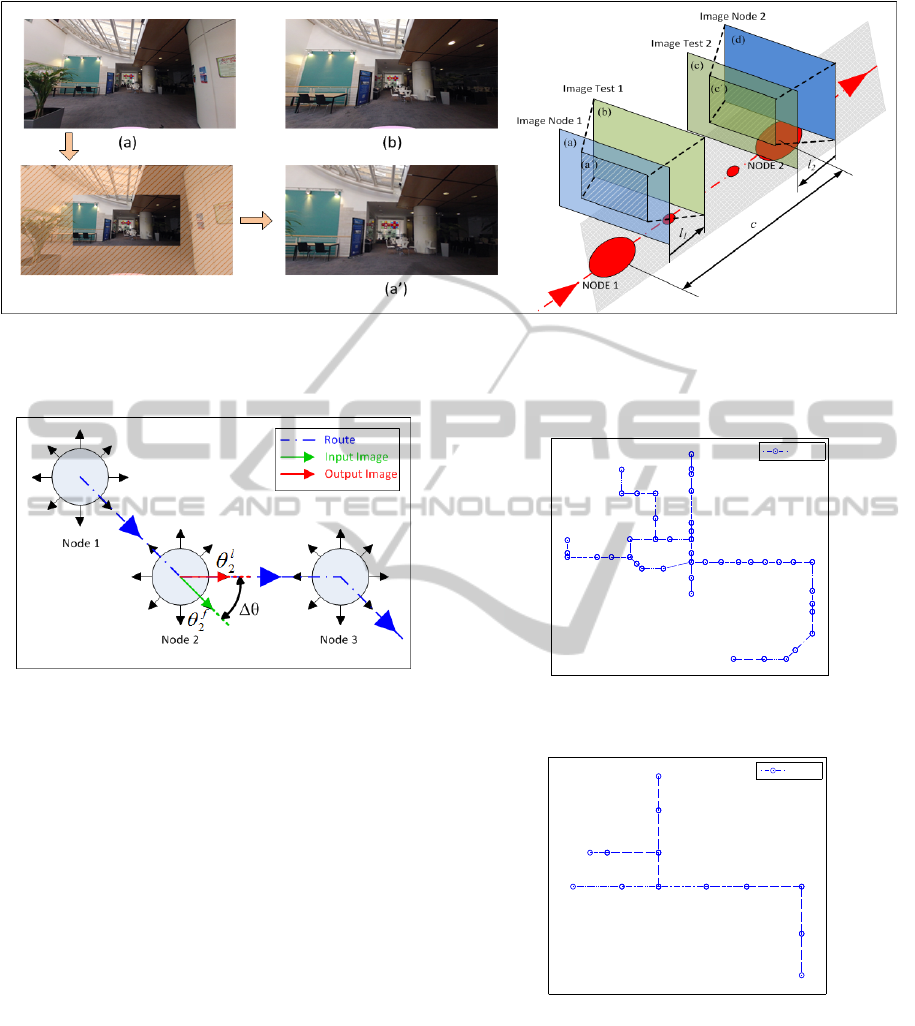
Figure 2: Example of two test images located in different relative positions regarding the closest node. (a) Image node 1, (a’)
Zoom-in of the Image Node 1, (b) Image Test 1, (c) Image Test 2, (c’) Zoom-in of the Image Test 2 and (d) Image Node 2. On
the right, it appears samples of the images (a), (a’) and (b) to show the zoom process and appearance similarity improvement.
l
1
and l
2
are topological distances between a node and a route image, and c the topological distance between nodes.
Figure 3: Phase change estimation in a node.
is the direction that the robot has to follow in order
to arrive to the next one. We estimate the phase lag
produced in a node as:
∆θ
i
= θ
l
i
− θ
f
i
(6)
In Fig. 3 we can see a graphical representation of
the phase change estimation in a node. We set the ori-
entation of the map by defining the direction of the
output image for the first node. That direction defines
the global orientation system of the map. After that,
the orientation of the graph is updated in every node
using ∆θ
i
. Although the map and the nodes use differ-
ent angle reference systems, it does not affect to the
results since we compute angle differences. Once we
have defined the global map orientation reference, we
can compute the phase lag with each node local ori-
entation system. That information will be used during
the path estimation task.
When a new route is studied, the algorithm ini-
tializes a new coordinates system. That route will
be analyzed independently of the global graph until
a common node is found. Using the position and ori-
entation of the common node regarding both systems,
Map 1
Nodes
(a)
Map 2
Nodes
(b)
Figure 4: Graph representation of the node’s arrangement
obtained with the map building algorithm for (a) Area 1 and
(b) Area 2.
we are able to add the new nodes to the global graph
correctly. If the path of a new route coincides with a
previous one, the topological distance c of the nodes
is estimated again, and the result included in the map
by calculating the mean with the previous values.
TopologicalMapBuildingandPathEstimationUsingGlobal-appearanceImageDescriptors
389

In Fig. 4 it is possible to see the map’s graph of (a)
the Area 1 and (b) the Area 2. In the experiments, we
use a high number of scales in order to increase the
precision in the topological distance estimation. In
particular, s
n
has a maximum value of 2.5 with a step
of 0.1, and s
r
reaches 1.4 with an increment of 0.05.
With that parameters, the time spent to make the nec-
essary comparisons per route image is 720 ms. We
can appreciate that the algorithm is able to estimate
the connections between nodes maintaining the ap-
pearance of the real layout of both areas. The Area 1
has been the most challenging due to the higher num-
ber of nodes, the transition from different rooms and
the loop in the map. The graph representation slightly
differs from the real layout, specially in the angle of
the right lower part nodes of the loop. Those nodes are
where the loop closure is produced, and the angle dif-
ference is due to the accumulated error in the distance
estimation of the nodes in the loop, not in the angle
estimation. Since the estimation of the phase lag be-
tween nodes is correct, the navigation is not affected
despite of the inaccuracy in the graph representation.
If there is not enough distance between adjacent
nodes, or the frequency of the route’s images is low,
a node might not be included in the graph, as the al-
gorithm does not find the necessary repetitions of the
node in the information vector when doing the node
retrieval. The system is especially sensitive in the
phase lag between nodes, since it is based on the an-
gle estimation of the input and output node’s images.
For that reason, it is advisable to raise the frequency
of the image acquisition in the nodes where there is a
change in the direction.
4 PATH ESTIMATION
ALGORITHM
Once we obtain the graph of the map, our follow-
ing objective is to estimate the path of the routes in
the map. This can be faced as a localization prob-
lem using visual information. If we base the local-
ization of the route just on the retrieval of the nearest
node’s images, our knowledge of the positions will
be limited to node’s location. In these experiments
we try to improve the localization extending it also to
intermediate points between map nodes. We use the
scale analysis of the images to carry out this task in
a similar way as seen in section 3. The algorithm
uses the adjacency matrix A and the map database
Z that includes the descriptors of the node’s images
obtained during the map building. The comparison
of the global-appearance descriptor of a route image
z
r
with Z provides a measurement of their similar-
ity with all the node’s descriptors using (3). On the
other hand, the matrix A contains information about
the topological distance of the matched nodes, mak-
ing it possible to find out the minimum topological
distance between two nodes of the map.
Once the descriptor z
r
of an image’s route has
been built, the first step consists in calculating the
Euclidean distance between it and the descriptors in-
cluded in the map database (i.e., the descriptors of the
node’s images). We obtain d
r
i
for i = 1. . . m. We iden-
tify each d with its corresponding node n, angle θ and
node image scale s
n
. Then, we classify the results re-
garding d. We select the k-nearest-neighbors, and re-
peat the experiments for different route images scales
s
r
. Specifically, we use k = 10 neighbors.
Next, we weight the image distance d of every se-
lected neighbor using their position and orientation.
The aim is to penalize the probability of neighbors
that are geometrically far from the last robot pose.
Since our classifier uses the minimum image distance
d as a criteria, we define a function that multiplies
the image distance of each neighbor regarding a fac-
tor that increases according to the topological distance
and phase lag.
To carry out this process, we first estimate the
topological distance between the position of the pre-
vious route image and every neighbor selected dur-
ing the matching. We are able to find out the shortest
path between two nodes using the information stored
in A. Since we have a connected graph, a path that
connects two nodes of the map can always be found.
Being c
n1,n2
the cost to traverse two adjacent nodes
n
1
, n
2
∈ A, and P
i, j
= [n
i
, . . . n
j
] the sequence of nodes
of the shortest path that connects n
i
and n
j
, the cost
C
i, j
associated with P
i, j
can be defined as:
C
i, j
=
n
j
∑
n
i
c
n
i
,n
i+1
(7)
being c
n
i
,n
i+1
the topological distance between ad-
jacent nodes defined in (5).
Our weighting function takes into account
changes in both position (nodes) and orientation.
Considering the image i−th of a route, the value of d
is updated as:
d
0
= d × [w
1
·C
i,i−1
+ w
2
· ∆θ
i,i−1
] (8)
w
1
and w
2
are weighting constants. Specifically,
w
1
is related with the topological distance, and w
2
weights changes in the path orientation. The function
updates the image distance d based on the topologi-
cal distance and phase lag between each neighbor and
the previous localization of the path. The multiplier
weighting term increases as the neighbors present
higher topological distance and orientation difference
ICINCO2013-10thInternationalConferenceonInformaticsinControl,AutomationandRobotics
390
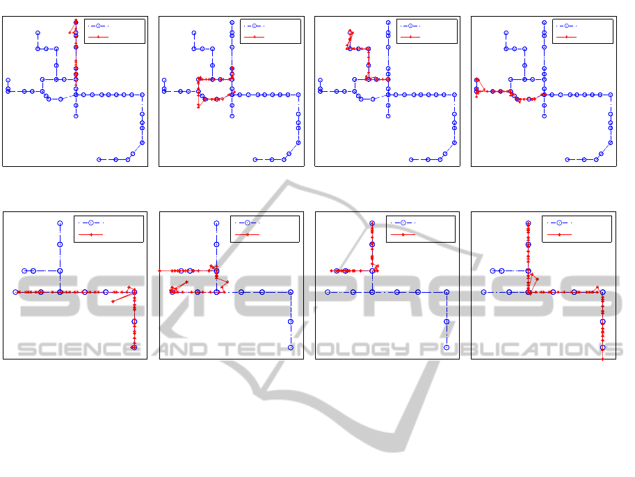
Map 1
Map
Route 1
(a)
Map 1
Map
Route 4
(b)
Map 1
Map
Route 6
(c)
Map 1
Map
Route 8
(d)
Map 2
Map
Route 1
(e)
Map 2
Map
Route 2
(f)
Map 2
Map
Route 3
(g)
Map 2
Map
Route 4
(h)
Figure 5: Path estimation of the (a) Route 1, (b) Route 4, (c) Route 6 and (d) Route 8 of the Area 1 over the created graph,
and path estimation of the (e) Route 1, (f) Route 2, (g) Route 3 and (h) Route 4 of the Area 2 over the created graph
regarding the last path location. By incrementing the
image distance of an experiment, we reduce its likeli-
hood of being chosen as nearest neighbor. That way,
the function penalizes important changes in position
and orientation between consecutive route scenes.
The multiplier term might change for each neighbor
of the current node, since the estimated nearest node
and orientation may vary in every particular case. We
determine the constants’ value experimentally. In our
function, we choose w
1
= 0.15 and w
2
= 0.1.
Once the image distances are updated, we classify
the selected experiments regarding d
0
, and choose the
Nearest Neighbor. As a result, we find out the closest
node n to the route image, its orientation θ, and the
scales of both the node’s image s
n
and the route’s im-
age s
r
. We have to take into account that θ must be
corrected with the phase lag between the map global
system and the node reference system, estimated pre-
viously in the map building. The current position of
the robot in the graph is estimated using the nearest
node and the relative position with that node (l) using
(1).
Figure 5 shows the path estimation of different
routes of the two areas. The dots in the route’s paths
represent the position of the different images studied.
The values of s
n
and s
r
have been determined experi-
mentally, being 2.2 the maximum scale with a step of
0.4 and 0.3 respectively. The time necessary to carry
out the localization of an input image is 330 ms.
We can compare the results with the synthetic
routes path representation in Fig. 1. As it can be seen,
the algorithm deals with the interpolation of the lo-
cation estimation in halfway positions of the nodes
using the image’s scales information. In general, the
location precision in changes of direction in the routes
decreases. It is also important that, despite the fact
that we introduce the weighing function, the algo-
rithm is capable of finding again the correct position
although a previous estimation is not correct, as we
can see in Fig. 5(a) and (c). The result in the path rep-
resentation of the fourth route of Area 1 (Fig. 5(b)) is
also interesting. As we can appreciate in Fig. 1(b),
the route 4 presents a path that differs from the layout
of the nodes, and the algorithm is able to estimate the
position accurately despite that fact.
Therefore, the results prove that our algorithm
deals with the estimation of the route path in inter-
mediate positions of the nodes and also deals false
association in former experiments of the route despite
using a weighting function.
TopologicalMapBuildingandPathEstimationUsingGlobal-appearanceImageDescriptors
391

5 CONCLUSIONS
In this paper we have studied the problem of topo-
logical map building and navigation using global-
appearance image descriptors. The map building al-
gorithm developed is able to estimate the relations be-
tween nodes and create a graph using the informa-
tion captured along some routes in the environment
to map. Moreover, we introduce a study of the im-
age’s scales in order to find out the topological dis-
tance between nodes which can be considered to ap-
proximately be proportional to the geometrical dis-
tance. The results present a high accuracy in the node
detection and estimation of its adjacency and relative
orientation as it can be seen in the graphs obtained
in the map building process. All that information ar-
ranges the representation of the map through a graph.
We have also created an algorithm which esti-
mates the path of routes along the area. It takes profit
of the image’s scale study to improve the location
with an interpolation of the route position between
nodes. The use of a weighting function to penalize
changes in position and orientation in consecutive im-
ages during the navigation improves the localization
accuracy. Despite that weight, the algorithm is able to
relocate the robot correctly although a previous image
of the route would introduce a false retrieval.
The results obtained both in the map building and
the path representation of routes encourage us to con-
tinue studying the possibilities of the application of
global-appearance image descriptors to topological
navigation tasks. It would be interesting to extend
this study in order to find the minimum information
necessary to make the navigation optimal, the appli-
cation of new global-appearance descriptors, or the
improvement in the phase estimation in order to make
the algorithm able to correct small errors in the orien-
tation.
ACKNOWLEDGMENTS
This work has been supported by the Spanish gov-
ernment through the project DPI2010-15308.
REFERENCES
Cummins, M. and Newman, P. (2009). Highly scalable
appearance-only SLAM - FAB-MAP 2.0. In Proceed-
ings of Robotics: Science and Systems, Seattle, USA.
Frizera, R., H., S., and Santos-Victor, J. (1998). Visual nav-
igation: Combining visual servoing and appearance
based methods.
Gaspar, J., Winters, N., and Santos-Victor, J. (2000).
Vision-based navigation and environmental represen-
tations with an omnidirectional camera. Robotics and
Automation, IEEE Transactions on, 16(6):890 –898.
Gil, A., Reinoso, O., Ballesta, M., Julia, M., and Paya,
L. (2010). Estimation of visual maps with a robot
network equipped with vision sensors. Sensors,
10(5):5209–5232.
Krose, B., Bunschoten, R., Hagen, S., Terwijn, B., and
Vlassis, N. (2007). Visual homing in enviroments with
anisotropic landmark distrubution. In Autonomous
Robots, 23(3), 2007, pp. 231-245.
Lowe, D. (2004). Distinctive image features from scale-
invariant keypoints. Int. J. Comput. Vision, 60(2):91–
110.
Menegatti, E., Maeda, T., and Ishiguro, H. (2004). Image-
based memory for robot navigation using properties
of omnidirectional images. Robotics and Autonomous
Systems, 47(4):251 – 267.
Moravec, H. and Elfes, A. (1985). High resolution maps
from wide angle sonar. In Robotics and Automation.
Proceedings. 1985 IEEE International Conference on,
volume 2, pages 116 – 121.
Murillo, A., Guerrero, J., and Sagues, C. (2007). Surf
features for efficient robot localization with omnidi-
rectional images. In Robotics and Automation, 2007
IEEE International Conference on, pages 3901 –3907.
Oliva, A. and Torralba, A. (2001). Modeling the shape of
the scene: a holistic representation of the spatial en-
velope. In International Journal of Computer Vision,
Vol. 42(3): 145-175.
Paya, L., Fenandez, L., Reinoso, O., Gil, A., and Ubeda,
D. (2009). Appearance-based dense maps cre-
ation: Comparison of compression techniques with
panoramic images. In 6th Int Conf on Informatics in
Control, Automation and Robotics.
Scaramuzza, D., Martinelli, A., and Siegwart, R. (2006). A
flexible technique for accurate omnidirectional cam-
era calibration and structure from motion. In Com-
puter Vision Systems, 2006 ICVS ’06. IEEE Interna-
tional Conference on, page 45.
Torralba, A. (2003). Contextual priming for object detec-
tion. In International Journal of Computer Vision, Vol.
53(2), 169-191.
Woodman Labs, I. (2013). http://gopro.com/hd-hero2-
cameras/.
ICINCO2013-10thInternationalConferenceonInformaticsinControl,AutomationandRobotics
392
