
SHARP: Shade-avoidance Response in Plants
An Evolutionary Simulation Software Package
Wen Fung Leong
1
, Sanjoy Das
1
, Stephen M. Welch
2
and Cynthia Weinig
3
1
Electrical & Computer Engineering Department, Kansas State University, Manhattan, KS, U.S.A.
2
Department of Agronomy, Kansas State University, Manhattan, KS, U.S.A.
3
Department of Botany, University of Wyoming, Laramie, WY, U.S.A.
Keywords: Evolution, Plant, Shade-avoidance, Simulation, Education, Matlab.
Abstract: Educational simulators take learning to the next level by bringing students’ understanding of a subject closer
to their personal experience. In this paper, software to simulate the evolution of shade-avoidance responses
in plants is developed. Models and equations to imitate the response are described. An example simulated
scenario is illustrated and discussed. This simulation demonstrates typical shade-avoidance response in
plants; the competition for sunlight between plants grown in high density conditions channelizes more
resources towards longer stems. Additionally, the simulations show how increased competition over plants
grown in low density conditions lowers the variability in the overall shapes of the individual plants.
1 INTRODUCTION
The increasing of computing power and its
decreasing cost has extended the development of
simulation-based educational and training tools to
various fields other than their traditional areas of
use, i.e. aviation (Kincaid and Westerlund, 2009).
Various types of educational simulation tools
depend on the specific fields and their objectives.
For instance, simulation games for teaching Political
Science (e.g., The Redistricting Game (USC
Annenburg Foundation, 2010)) aims to provide
understanding on the mechanics of the real world
political systems; the typology of medical simulation
tools proposed in (Alinier, 2007) aims to develop
students’ cognitive, psychomotor and interpersonal
skills, and to enhance their experiences with the
ultimate goal of saving lives and ensuring patients’
well-being; and another visualization tool
(Kethireddy and Suthaharan, 2004) helps students to
understand the difficult concepts of computer
networks.
In the fields of biology, (Tinker and Mather,
1993)’s interactive genetic simulation software can
be an educational tool for undergraduate students to
learn genetics, selection, the process of meiosis, and
phenotypes. The authors in (Martin and Skavaril,
1984), (Fita et. al., 2010) developed a computer
simulation program to teach students the concepts in
plant breeding, including genetic drift, the steps
involved in various breeding methods and the
development of different lines. The authors in
(Martin and Skavaril, 1984), (Fita et. al., 2010)
pointed out that plant breeding simulations allow
students to experience the whole plant breeding
process as an “actual” plant breeder and at the same
time gained their interest in this field.
Inspired by their works (Tinker and Mather,
1993), (Martin and Skavaril, 1984), (Fita et. al.,
2010), a simple educational simulation program to
simulate the evolution of shade-avoidance responses
in plants is proposed. The program will demonstrate
the major shade-avoidance traits as they change over
multiple generations. An evolutionary algorithm
(Deb, 2001), (Engelbrecht, 2007) is used to imitate
the biological processes of the plants. The
immediate intended users are science teachers in a
summer training institute.
2 SHADE AVOIDANCE
RESPONSES IN PLANTS
Plants have the ability to survive in various
environmental conditions. At high population
densities plants compete with their neighbors for
limited resources such as water, nutrients, and
163
Fung Leong W., Das S., M. Welch S. and Weinig C..
SHARP: Shade-avoidance Response in Plants - An Evolutionary Simulation Software Package.
DOI: 10.5220/0004485801630170
In Proceedings of the 3rd International Conference on Simulation and Modeling Methodologies, Technologies and Applications (SIMULTECH-2013),
pages 163-170
ISBN: 978-989-8565-69-3
Copyright
c
2013 SCITEPRESS (Science and Technology Publications, Lda.)
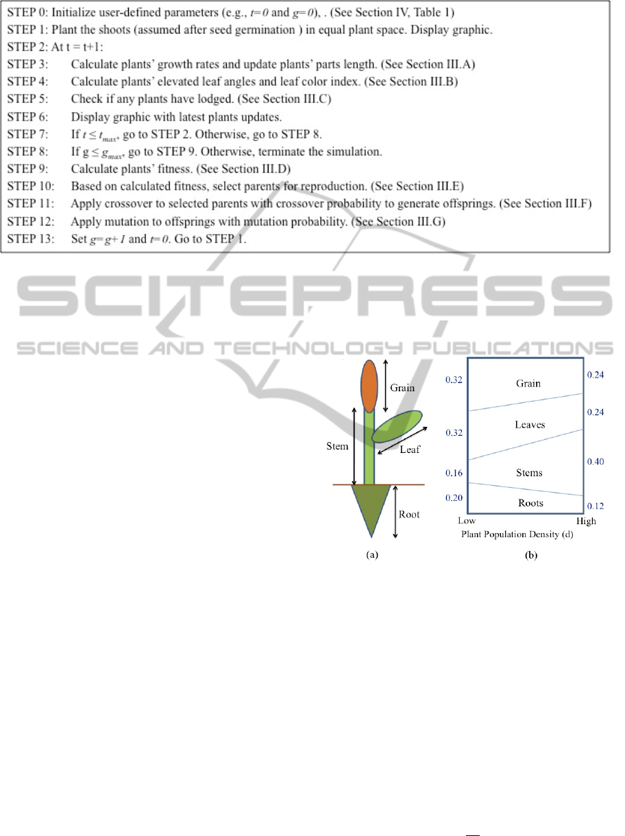
Figure 1: Pseudocode of the SHARP evolutionary simulation software package.
especially sunlight (Casal, 2012), (Franklin and
Whitelam, 2005), (Sasidharan et. al., 2010),
(Keuskamp and Pierik, 2010), (De Wit et. al. 2012).
In competing for sunlight, plants utilize
photosensitive molecules in their leaves to sense red
(R) and far-red (FR) wavelengths; the R:FR ratio is
an indicator of nearby neighboring plants (De Wit et.
al., 2012). A low R:FR ratio indicates shading by
other plants and induces shade-avoidance response
to secure more sunlight (i.e. light interception). The
phenotypic traits that constitute the shade-avoidance
response include stem elongation, petiole elongation,
reduction of chlorophyll concentration, and leaf
hyponasty (i.e. increase in leaf elevation angle)
(Casal, 2012), (Franklin and Whitelam, 2005),
(Sasidharan et. al., 2010), (Keuskamp and Pierik,
2010), (De Wit et. al., 2012). Plants under long-term
shading exhibit traits that are related to shade-
avoidance syndrome (SAS). These include reduced
branching and acceleration of flowering (albeit with
fewer seeds) to ensure reproduction (Sasidharan et.
al., 2010). Thus, in agriculture, plants undergoing
shade-avoidance syndrome will results in a lowered
crop yield.
3 THE FRAMEWORK OF THE
SIMULATION PROGRAM
The proposed simulation tool assumes there are no
water and nutrient limitations; the simulated shade-
avoidance phenotypic traits are stem elongation, leaf
elevation angle, reduction of chlorophyll
concentration, reduced root size and shorter leaf
length (Casal, 2012), (Franklin and Whitelam,
2005). The pseudocode of the simulated program is
presented in Figure 1. Parameters and variables will
be elaborated in the next Section.
Figure 2: (a) Specification of a plant with arrows
represents the length of a specific plant part. (b) Shade-
avoidance response graph with x-axis represents the plant
population density.
3.1 Plant Growth Model
For visualization, every plant has one root mass, a
stem, two leaves, and a grain mass. As depicted in
Fig 2(a), the lengths of these plant parts (i.e. Grain,
Stem, Root, and Leaf) are approximated via Euler
integration. At current generation denoted as g and
current day denoted as t, the plant parts’ lengths for
plants i = 1, …, N are updated via (1a) to (1d):
,∆
,
∆
,
(1a)
SIMULTECH2013-3rdInternationalConferenceonSimulationandModelingMethodologies,Technologiesand
Applications
164

,∆
,
∆
,
1b
,∆
,
∆
,
1c
,∆
,
∆
,
1d
In the above equations, the time increment Δt is
equal to 1 day. The derivative terms above that
represent the growth rate (changes of length each
unit time) of each given plant part, are as follows:
,
1
,
(2a)
,
1
,
(2b)
,
1
,
(2c)
,
1
,
(2d)
Subject to:
1
,
,1
,
,1
,
,1
,
0
(2e)
The equations in (2) model the growth rate of each
plant part as proportional to the light interception per
day per leaf, a proxy for rate of photosynthesis, and
to a factor (i.e. (1 + ε)) defining the fraction of each
new increment of photosynthate that is allocated to
each tissue type.
The variables A’s (i.e. A
G
, A
S
, A
R
, and A
L
) in (2)
are the allocation factors of photosynthate (i.e. the
product of photosynthesis). They are determined by
the user-defined plant population density parameter,
d value that is represented by the x-axis of the
shade-avoidance response graph in Fig.2b. As
shown in Fig. 2b, the range of the d values is low to
high densities. If d is a high value (crowded
conditions), the graph depicts the shade-avoidance
traits of stem elongation, reduced root size and
lowered seed production relative to plants grown in
uncrowded conditions. The range of d is set as
[0.001,1] for this framework. The equations to
calculate the A values are derived from the graph
and are presented in (3a) to (3d) below:
0.32
1
0.24
(3a)
0.16
1
0.40
(3b)
0.20
1
0.12
(3c)
0.32
1
0.24
(3d)
The variable, L
I
in (2) is the light intercepted by the
leaf in one day, representing a proxy for rate of
photosynthesis. It is equal to the angle θ (see Fig. 3)
multiplied by the plant leaf’s area. The angle θ is
defined from the plant’s leaf node to the maximum
heights of its nearest neighboring plants, and the
maximum degree is 180° or π (in radians). The
rationale is that the plant’s leaf can only receive
sunlight when the sun is above the horizon and the
amount received in a day will be proportional to the
time it is not shaded; that is, the time during which
the sun is within the subtended angle. In this
program, the assumption is that the leaves have unit
area and receive θ (in radians) of sunlight, i.e. L
I
= θ.
The four ε’s (i.e. ε
G
, ε
S
, ε
R
and ε
L
) values (or the four
“loci”) in (2) represent the genetic makeup of a
plant, meaning each plant has four genes. Every
plant has different set of ε values that mimic the
genetic variation between plants. Lastly, the fixed
parameters, k’s (i.e. k
G
, k
s
, k
R
, and k
L
) in (2) are plant
part growth rated adjustment factors set by experts
to improve simulation realism.
Figure 3: An illustration of plant 2 (i.e. i=2) and its nearest
neighboring plants, plant 1 and plant 3. The angle θ
represents the amount of sunlight exposed by plant 2 and
angle α is the leaf elevation angle.
3.2 Leaf Specifications
The above SHARP model focuses on variable
growth rates of plant parts reared in a high-density
environment. The larger stem allocation factor at
high density (Fig. 2b) leads to increasing plant
height under shading. Other traits such as elevated
leaf angle and reduced chlorophyll concentration are
two of the responses that aim to “elevate leaves
towards unfiltered daylight and provide an essential
survival strategy in rapidly growing population”
(Franklin and Whitelam, 2005).
This model incorporates the elevated leaf angle
calculate via the following equation:
SHARP:Shade-avoidanceResponseinPlants-AnEvolutionarySimulationSoftwarePackage
165

,
1
2
,1
1
2
0.8333
5
180
(4)
Equation (4) has two roles. First, it maps the angle α
in radians (See Fig.3) to the biological elevated leaf
angle, which ranges from 5 degree to 80 degree
(Sasidharan et. al., 2010), (Keuskamp and Pierik,
2010), (De Wit et. al., 2012), (Hammer et. al., 2009).
These are rough estimates garnered from several
articles not necessarily representative of any single
species. However, the range serves the purpose of
demonstrating how plants respond to shade in
crowded environments. The second role is to adjust
the elevated leaf angle by taking the average of the
leaf angle calculated from the previous day (i.e. t-1)
and the current day (i.e. t) to avoid any
unrealistically sudden changes of elevated leaf angle
that will be displayed on the graphic.
The changes in chlorophyll concentrations are
depicted in different levels of green color. The
darker green color represents leaf with high
chlorophyll content; while the lighter green color
represents the opposite. In this program, we use a
color index to represent different levels of green
listed in a look-up table. Currently, the look-up table
has seven green shades. From darkest to lightest,
they are: Dark Green, Forest Green, Dark Sea Green,
Medium Sea Green, Lime Green, Lawn Green, and
Green Yellow. These articles (10, Keuskamp and
Pierik, 2010) , (Smith and Whitelam, 1997) stated
the reduction in chlorophyll production due to lack
of light is commonly observed in leaf development
during shade-avoidance. To model this trait, we
borrow the idea of mapping the leaf angle α in
radians to the leaf color index in Equation( 4); the
model is formulated as the following:
,1
1
2
,1
1
2
3.91971
(5)
3.3 Plant Lodging
In nature, there are multiple sources of plant
mortality. In this program, the only source is plant
lodging – the plant falls over if it becomes top-heavy
relative to its root mass. The threshold probability of
lodging (P
Lodge
) in one-day period is calculated by
the following equations:
,
,
1
,
(6a)
where,
,
,
,
,
(6b)
In the above equation, k
Lodge
is a fixed parameter that
is set to a large enough value to insure that the
effects of lodging are clear to learners. Plant i’s
chances to survive the next day will be decided
when a uniform random number, r is greater or
equal to P
Lodge
(i.e. r ≥ P
Lodge
). Smaller k
Lodge
value
will lower the P
Lodge
, thus allowing the plants to
survive longer period of days.
3.4 Plant Fitness
Generation times were set to t
max
=120 days. At day
120, the surviving plants’ ability to produce the
amount of seeds after pollination is the metric for
plants’ fitness. In this model, the length of each
grain plant part is an indicator of fitness. The fitness
calculation for surviving plants i = 1, …, N
Survive
is
given in (7) below:
, 120
, 120
∑
,120
(7)
3.5 Selection Scheme
This program implemented roulette-wheel selection
(Deb, 2001) in which the probability of reproducing
is proportional to fitness. This method has two
advantages: 1) Plants with high fitness are likely to
be selected but there is also some chance that they
won’t be selected; and 2) Due to its randomness,
plants with low fitness may be selected giving a
chance to preserve certain genes that are associated
with better traits.
3.6 Crossover Operator
The real-valued blend crossover operator (BLX-α)
(Deb, 2001); (Engelbrecht, 2007); (Eshelman and
Schaffer, 1993) is implemented to simulate cross-
pollination. Firstly, two surviving plants are selected
as parents 1 and 2. Next, the crossover operator ((8)
and (9)) is applied to the parental loci j with
crossover probability (pc) and to generate a plant
offspring’s (or seed’s) loci j that contains both the
parents’ genetic materials. If the crossover
probability isn’t met, the offspring’s (or seed’s) loci
j is copied directly from one of the parents’ loci j.
1
,120
,120
(8)
SIMULTECH2013-3rdInternationalConferenceonSimulationandModelingMethodologies,Technologiesand
Applications
166

12
0,1
(9)
Here, α, an user-defined parameter is an exploration
coefficient and α ≥ 0. The rand(0,1) represents the
uniformly distributed random number generator with
the range of 0 and 1. The
j
o
,
j
1
and
j
2
values
represent the offsping’s, parent 1’s, and parent 2’s
loci j respectively. The pc parameter is set to 0.5,
meaning there is a 50% chance for recombination to
happen. There are total of four loci for each
offspring. Self-pollination (or “selfing” occurs if the
plant offspring has the exact same four ε values as
its parent plant.
3.7 Mutation Operator
After plant offspring are produced, a mutation
operation is applied to locus j of each new individual
with mutation probability (pm). A Gaussian
distribution mutation operator (Deb, 2001) is utilized
for this step.
0,
(10)
Here,
j
o
represent the offspring’s loci j, N(0,σ
2
)
denotes a zero-mean Gaussian probability
distribution with variance, σ
2
. The parameter σ is set
to 0.005 and pm set to 0.01 (i.e. 1% chance for a
mutation event to happen).
4 SIMULATIONS
This section illustrates the visualization and output
generated by the simulation program. Table 1
contains parameters that require user-defined
settings. The k values and lodge weighting are not
shown as they are not accessible to users.
Table 1: SHARP parameter settings.
Parameter Name
Value
High
Density
Low
Density
Maximum generation
(g
max
)
25 25
Maximum number of
days (t
max
)
120 120
Ground length (meter) 8 48
d parameter (Figs. 2(b)) 0.9 0.1
Number of plants 16 16
Crossover probability (pc) 0.5 0.5
alpha parameter (α) 0.0 0.0
Mutation probability (pm) 0.01 0.01
Fig.s 4 and 5 are the examples of simulated
plants graphics. Both consist of two panels: panel (a)
illustrates a high population density environment;
panel (b) is low population density. The plants are
aligned uniformly (i.e. equal initial distances
between neighboring plants). Current generation and
days after planting information are displayed on the
top left of panel (b). Although 16 plants are
simulated in both conditions, panel (b) only
illustrates five plants to demonstrate plants in non-
crowded environment versus those living in crowded
environment. At 120 days in every generation, two
tables report the highest and lowest fitness values,
along with their corresponding ε values (i.e. genes).
See Fig. 5 for an example. Only roots are shown to
designate plants that have lodged. Students can
observe the effects of crowding on the plants’
behavior to compete for sunlight during their growth
period and how this behavior changes as the number
of generation increases. They can compare the
resulting plant traits in the two different
environments (e.g. plant height, elevated leaf angle,
chlorophyll content and root mass in every
generation).
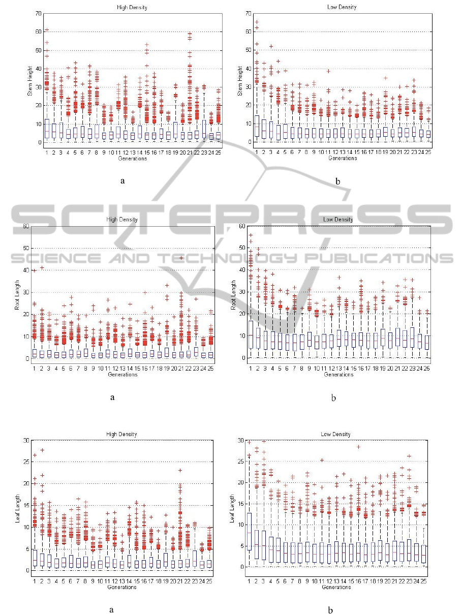
The simulated is run 50 times (i.e. 50 in silico
experiments) to gather enough data to plot the
distributions of the simulated plant traits in every
generation. The distributions are presented in box-
plots as shown in Figs. 6-9. In Fig 6(b), plants tend
to inherit larger grain size (i.e. yield more seed) in
the less densely populated area while in the crowded
environment (Fig. 6(a)), majority of the plants’ trait
with smaller grain size (i.e. lower yield) is more
prevalent, indicating plants will produce offspring to
be adaptable to shade-avoidance responses and
survive in such environment. There are outliers in
both plots. They indicate variability and diversity of
plants’ trait that may due to mutated genes or other
unexpected factors such as neighboring plants lodge
and that affected the plants’ response to growth. Figs
7(b) illustrates the majority of the plants’ stem
heights maintain almost consistent lower and upper
quartiles (or consistent distribution shapes) starting
from the 8
th
generation. This shows the majority of
the plants do not need to compete for sunlight in the
less crowded environment. On the other hand, Fig
7(a) shows the variability of distributions in some
generations, reflecting some plants were competing
in response to shade-avoidance and increase stem
height to get access to more sunlight. Fig 8(a)
clearly shows smaller plants’ root mass in the
crowded environment due to every plant compete for
limited water resource; while the large root mass is
more prevalent for plants growing in the low density
SHARP:Shade-avoidanceResponseinPlants-AnEvolutionarySimulationSoftwarePackage
167
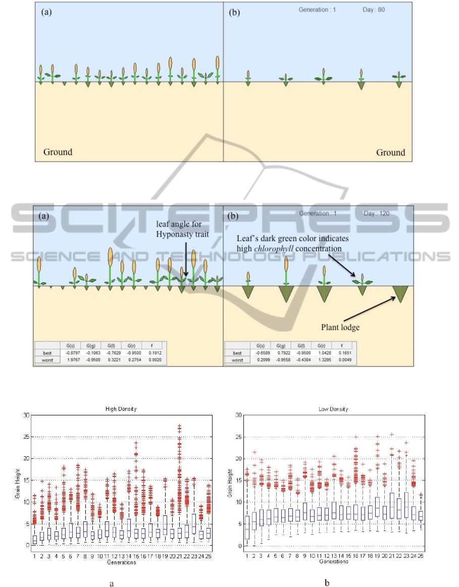
Figure 4: Illustration of the plants status growing in (a) high and (b) low population density at first generation and 80 days
after planting.
Figure 5: Illustration of the plants status after 120 days of planting at first generation.
Figure 6: Box plots of grain height in two plant growing conditions in the period of 25 generations for 50 test runs.
SIMULTECH2013-3rdInternationalConferenceonSimulationandModelingMethodologies,Technologiesand
Applications
168
.
Figure 7: Box plots of stem height in two plant growing conditions in the period of 25 generations for 50 test runs.
Figure 8: Box plots of root length in two plant growing conditions in the period of 25 generations for 50 test runs.
Figure 9: Box plots of leaf length in two plant growing conditions in the period of 25 generations for 50 test runs.
SHARP:Shade-avoidanceResponseinPlants-AnEvolutionarySimulationSoftwarePackage
169

environment (see Fig. 8(b)). Plants grown in the
wide-open space tend to produce larger leaves length
with higher variability (in Fig. 9(b)). This isn’t the
case for plants grow in crowded condition. As
illustrated in Fig. 9(a), majority of the plants
continue to produce offspring with small leaf length,
a trait reflects receiving lesser sunlight.
5 FUTURE WORK
The above modeling framework shows the potential
of developing a simulated educational program to
educate students about shade-avoidance responses in
plants. Several improvements will be implemented
to bring the simulated response closer to nature. For
example, one improvement is to define the leaf area
equation and make light interception proportion to
leaf area. Another idea is to transfer this program
into graphic user interface (GUI), allowing students
play with the parameters to create different
experimental scenarios, learn, and observe the
simulated results (i.e. plants’ responses).
ACKNOWLEDGEMENTS
This research was supported through NSF Grant No.
0923752 to Weinig (PI), McClung, Welch, Das &
Maloof (co-PIs).
REFERENCES
Kincaid J. P. and Westerlund K. K., 2009. Simulation in
education and training, IEEE Proceedings of the 2009
Winter Simulation Conference (WSC), 273 – 280.
USC Annenburg Foundation, accessed December 19,
2012. The ReDistricting Game. Virginia Civics, Item
#273. available: http://vagovernmentmatters.org/web-
resources/273
Alinier G., 2007. A typology of educationally focused
medical simulation tools. Medical Teacher, 29(8),
243-250.
Kethireddy J. and Suthaharan S., 2004. Visualization
Teaching Tool for Simulation of OSI Seven Layer
Architecture. IEEE Proceesings in SoutheastCon, 335-
342.
Tinker N. A. and Mather D. E., 1993. GREGOR: software
for genetic simulation. Journal of Heredity, 84(3),
237-237.
Martin S. K. St. and Skavaril R.V., 1984. Computer
simulation as a tool in teaching introductory plant
breeding. Journal of Agronomic Education, 13, 43-47.
Fita A., Tarín N., Prohens J., and Rodríguez-Burruezo A.,
2010. A software tool for teaching backcross breeding
simulation. HortTechnology, 20(6), 1049-1053.
Deb K., 2001. Multi-Objective Optimization Using
Evolutionary Algorithms, 1st edn, John Wiley & Sons,
England, p. 123.
Engelbrecht A. P., 2007. Computational Intelligence: An
Introduction; John Wiley & Sons, England, p. 148-149
Casal J. J., 2012. Shade avoidance; Arabidopsis Book, 10,
ch. e0157, p. 1-19.
Franklin K. A. and Whitelam G. C., 2005. Phytochromes
and shade-avoidance responses in plants. Annals of
Botany, 96(2), 169-175.
Sasidharan R., Chinnappa C. C., Staal M., Elzenga J. T.
M., Yokoyama R., Nishitani K., Voesenek L. A.C.J.,
and Pierik R., 2010. Light quality-mediated petiole
elongation in Arabidopsis during shade avoidance
involves cell wall modification by xyloglucan
endotransglucosylase/hydrolases. Plant physiology,
154(2), 978-990.
Keuskamp D. H. and Pierik R., 2010. Photosensory cues
in plant–plant interactions: regulation and functional
significance of shade avoidance responses. Plant
Communication from an Ecological Perspective, 159-
178.
De Wit M., Kegge W., Evers J. B., Vergeer-van Eijk M.
H., Gankema P., Voesenek L. A. C. J., and Pierik R.,
2012. Plant neighbor detection through touching leaf
tips precedes phytochrome signals. Proceedings of the
National Academy of Sciences, 109(36), 14705-14710.
Hammer G. L, Dong Z., McLean G., Doherty A., Messina
C., Schussler J., Zinselmeier C., Paszkiewicz S., and
Cooper M., 2009. Can changes in canopy and/or root
system architecture explain historical maize yield
trends in the US corn belt? Crop Science, 49(1), 299-
312.
Smith H. and Whitelam G. C., 1997. The shade avoidance
syndrome: multiple responses mediated by multiple
phytochromes. Plant, Cell atid Environment, 20, 840-
844.
Eshelman L. J. and Schaffer J. D., 1993. Real-Coded
Genetic Algorithms and Interval-Schemata.
Foundations of Genetic Algorithms, 2, 187-202.
SIMULTECH2013-3rdInternationalConferenceonSimulationandModelingMethodologies,Technologiesand
Applications
170
