
Subspace Clustering with Distance-density Function and Entropy in
High-dimensional Data
Jiwu Zhao and Stefan Conrad
Institute of Computer Science, Databases and Information Systems,
Heinrich-Heine University, Universitaetsstr. 1, 40225 Duesseldorf, Germany
Keywords:
Subspace Clustering, Density, High dimensionality, Entropy.
Abstract:
Subspace clustering is an extension of traditional clustering that enables finding clusters in subspaces within
a data set, which means subspace clustering is more suitable for detecting clusters in high-dimensional data
sets. However, most subspace clustering methods usually require many complicated parameter settings, which
are almost troublesome to determine, and therefore there are many limitations in applying these subspace
clustering methods. In our previous work, we developed a subspace clustering method Automatic Subspace
Clustering with Distance-Density function (ASCDD), which computes the density distribution directly in high-
dimensional data sets by using just one parameter. In order to facilitate choosing the parameter in ASCDD
we analyze the relation of neighborhood objects and investigate a new way of determining the range of the
parameter in this article. Furthermore, we will introduce here a new method by applying entropy in detecting
potential subspaces in ASCDD, which evidently reduces the complexity of detecting relevant subspaces.
1 INTRODUCTION
We usually need to investigate unknown or hidden
information from raw data. Clustering techniques
help us to discover interesting patterns in the data
sets. Clustering methods divide the observations into
groups (clusters), so that observations in the same
cluster are similar, whereas those from different clus-
ters are dissimilar. The clustering is important for data
analysis in many fields, including market basket anal-
ysis, bio science, and fraud detection.
Unlike traditional clustering methods, which seek
clusters only in the whole space, subspace cluster-
ing enables clustering in particular projections (sub-
spaces) within a data set. Subspace clustering is usu-
ally applied in high-dimensional data sets.
Many famous subspace clustering algorithms can
find clusters in subspaces of the data set. However, the
effectivity is a problem of these algorithms. For in-
stance, it is commonly known that the majority of the
algorithms usually demand many parameter settings
for subspace clustering. In addition, the determina-
tion of the input parameters is not simple. Further-
more, varying many sensitive parameters often cause
very different clustering results.
In our former work, we introduced a density-based
subspace clustering algorithm ASCDD (Automatic
Subspace Clustering with Distance-Density function)
(Zhao and Conrad, 2012). With its density function,
the distribution of data is calculated directly in any
subspace, and clusters are automatically explored ac-
cording to the sizes of clusters. The method can be
applied for differently scaled data. Moreover, the al-
gorithm uses one parameter, which simplifies the ap-
plication process. In this paper, we investigate the
range of the parameter, in order to set the parameter
in a proper range. Another important improvement of
ASCDD is that we introduce an entropy based sub-
space search.
The remainder of this paper is organized as fol-
lows: In section 2, we present related work in the area
of subspace clustering and some ideas from other al-
gorithms. Section 3 describes the subspace cluster-
ing method ASCDD and presents our new ideas about
choosing the parameter and subspace detection with
entropy. Section 4 presents experimental studies for
verifying the proposed method. Finally, section 5 is
the conclusion of the paper.
2 RELATED WORK
In recent years, there has been an increasing amount
of literature on subspace clustering. Surveys con-
14
Zhao J. and Conrad S..
Subspace Clustering with Distance-density Function and Entropy in High-dimensional Data.
DOI: 10.5220/0004486600140022
In Proceedings of the 2nd International Conference on Data Technologies and Applications (DATA-2013), pages 14-22
ISBN: 978-989-8565-67-9
Copyright
c
2013 SCITEPRESS (Science and Technology Publications, Lda.)

ducted by (Parsons et al., 2004) and (Kriegel et al.,
2009) have divided subspace clustering algorithms
into two groups: top-down and bottom-up. Top-
down methods (e.g. PROCLUS (Aggarwal et al.,
1999), ORCLUS (Aggarwal and Yu, 2000), FINDIT
(Woo et al., 2004), COSA (Friedman and Meulman,
2004)) use multiple iterations for improving the clus-
tering results. Bottom-up methods (e.g. CLIQUE
(Agrawal et al., 1998), ENCLUS (Cheng et al., 1999),
MAFIA (Goil et al., 1999), CBF (Chang and Jin,
2002), DOC (Procopiuc et al., 2002)) firstly find clus-
ters in low-dimensional subspaces, and then expand
the searching into high dimensions. Other surveys
from (M
¨
uller et al., 2009) and (Sim et al., 2012) cat-
egorize the basic subspace clustering methods gener-
ally into grid-based, clustering-oriented and density-
based approaches.
The grid-based subspace clustering algorithms
partition the data space into cells with grids, and gen-
erate subspace clusters by combining dense cells with
big amount of objects. CLIQUE (Agrawal et al.,
1998) is a typical representation of grid-based sub-
space clustering algorithms. It detects firstly one-
dimensional subspace clusters, and combines them
to find high-dimensional subspace clusters. CLIQUE
has many extensions, one of them is ENCLUS (Cheng
et al., 1999), which measures the entropy values for
detecting potential subspaces with clusters, namely a
subspace with clusters has lower entropy than a sub-
space without clusters. The entropy calculation re-
quires density which is calculated as follows: Each
dimension is divided into cells, and the density is the
proportion of objects contained in a cell to all objects.
After detecting all the subspace candidates, the clus-
tering process is similar to CLIQUE.
A clustering-oriented subspace clustering method
assigns objects to k medoids (similar to k-means
(MacQueen, 1967)) to form clusters with correspond-
ing subspace. Representations of clustering-oriented
subspace clustering methods are PROCLUS and its
extensions, such as ORCLUS, FINDIT.
Many density-based subspace clustering ap-
proaches are based on the technique of DBSCAN (Es-
ter et al., 1996). For example, SUBCLU (Kr
¨
oger
et al., 2004) as an extension of DBSCAN is in-
tended for subspace clustering. The density of an
object is counted by the number of objects in a ε-
neighborhood. A cluster in a relevant subspace sat-
isfies two properties: All objects within a cluster are
density-connected with each other; If an object is
density-connected to any object of a cluster, it belongs
to the cluster as well.
Another density-based clustering technique such
as DENCLUE (Hinneburg et al., 1998) and DEN-
CLUE 2.0 (Hinneburg and Gabriel, 2007) use Gaus-
sian kernel function as the abstract density function
and apply hill climbing method to detect cluster cen-
ters. It is unnecessary to estimate numbers or posi-
tions of clusters, because clustering is based on the
density of each point. However, the estimation of pa-
rameters such as mean and variance in DENCLUE
or the iteration threshold and the percentage of the
largest posteriors in DENCLUE 2.0 is still necessary.
Almost all the mentioned subspace clustering
methods suffer from serious limitations of deter-
mining appropriate values of parameters. For in-
stance, the parameters such as the numbers of clus-
ters and subspaces of top-down methods; the bottom-
up method’s parameters, e.g. density, grid interval,
and size of clusters. These parameters influence the
iterations or clustering results, but the parameters are
difficult to be determined. In order to make the sub-
space clustering task more practical, it is necessary to
simplify the parameters.
With the motivation of facilitating the determina-
tion of parameters, a subspace clustering method AS-
CDD (Automatic Subspace Clustering with Distance-
Density function) was introduced in our previous
work. ASCDD can be applied directly in any sub-
space for searching clusters. Based on the density
values calculated with its density function, the centers
of clusters can be found easily. The idea of using a
density function is inspired by DENCLUE. However,
the definitions of the density functions are different.
ASCDD’s density function can be applied directly on
any subspace. A cluster in ASCDD is explored by
expanding neighbors of an object with high density.
Nevertheless, the definition and searching “density-
connected” neighbors are totally different from DB-
SCAN. The clustering process in ASCDD needs just
one parameter called DDT (distance-density thresh-
old) with the function of determining whether two ob-
jects are neighbors (belong to the same cluster). Since
choosing a proper DDT is important for ASCDD, in
this paper we investigate thoroughly the relation be-
tween setting the parameter DDT and the clustering
results and develop a way to set the range of DDT.
Although ASCDD can be applied on any subspace
directly, it is still required an effective way of choos-
ing the right subspaces with potential clusters instead
of searching each subspace. Our solution is to ap-
ply entropy on detecting the potential subspaces and
to reduce the subspace searching complexity. Unlike
ENCLUS, ASCDD’s entropy is not calculated by ap-
plying grids, but with the help of ASCDD’s density
function. The “interesting subspaces” in ENCLUS
are the subspaces with entropy that exceeds a parame-
ter ω. Meanwhile, interest gain more than a threshold
SubspaceClusteringwithDistance-densityFunctionandEntropyinHigh-dimensionalData
15
ε. However, the difficulty is to choose the proper pa-
rameters for an unfamiliar data set. In order to ap-
ply entropy more simply we use another technique
to locate significant subspace. The extension of en-
tropy makes ASCDD more efficient by detecting clus-
ters directly in subspace candidates. More details are
shown in the following sections.
3 AUTOMATIC SUBSPACE
CLUSTERING WITH
DISTANCE-DENSITY
FUNCTION (ASCDD)
Generally, a data set could be considered as a pair
(A,O), where A = {a
1
,a
2
,·· · } is a set of all at-
tributes (dimensions) and O = {o
1
,o
2
,·· · } is a set of
all objects. o
a
j
i
denotes the value of an object o
i
on
dimension a
j
.
A subspace cluster S is also a data set and can be
defined as follows:
S = (
e
A,
e
O)
where the subspace
e
A ⊆ A and
e
O ⊆ O, and S must
satisfy a particular condition C , which is defined dif-
ferently in each subspace clustering algorithm. How-
ever, a general principle of C is that objects in the
same cluster are similar, meanwhile the objects from
different clusters are dissimilar. S
e
A
indicates all sub-
space clusters that refer to
e
A.
Suppose S
1
,S
2
are two subspace clusters, where
S
1
= (A
1
,O
1
) and S
2
= (A
2
,O
2
), the intersection of
two subspace clusters is defined as follows: S
1
∩ S
2
=
(A
1
∪ A
2
,O
1
∩ O
2
)
The subspace, objects and subspace clusters have
following relations:
• If A
1
6= A
2
∨ O
1
6= O
2
=⇒ S
1
6= S
2
, the subspace
clusters that have different subspaces or objects
are considered as different ones.
• If A
1
⊇ A
2
∧ O
1
= O
2
or A
1
= A
2
∧ O
1
⊇ O
2
=⇒
S
1
> S
2
. So if S
1
> S
2
> ··· > S
n
, normally only
the largest subspace cluster S
1
is considered as a
clustering result.
The Automatic Subspace Clustering with
Distance-Density function (ASCDD) is based on its
density function. The following definitions are im-
portant for the density function. The distance-density
of objects o
i
and o
j
with regard to subspace
e
A is
defined as follows:
d
e
A
o
i
,o
j
=
1
(r
e
A
o
i
,o
j
2
· |O| + 1)
2
(1)
where r
e
A
o
i
,o
j
is the normalized Euclidean dis-
tance, which is calculated as follows: r
e
A
o
i
,o
j
=
s
∑
∀a∈
e
A
( ¯o
a
i
− ¯o
a
j
)
2
. The normalization of an object o
i
in one dimension a is defined as ¯o
a
i
=
o
a
i
−min(o
a
)
max(o
a
)−min(o
a
)
,
so ¯o
a
i
∈ [0, 1].
The density of an object o
i
relating to all objects
in subspace
e
A is defined as follows:
D
e
A
o
i
=
∑
∀o
j
d
e
A
o
i
,o
j
=
∑
∀o
j
1
r
e
A
o
i
,o
j
2
· |O| + 1
2
(2)
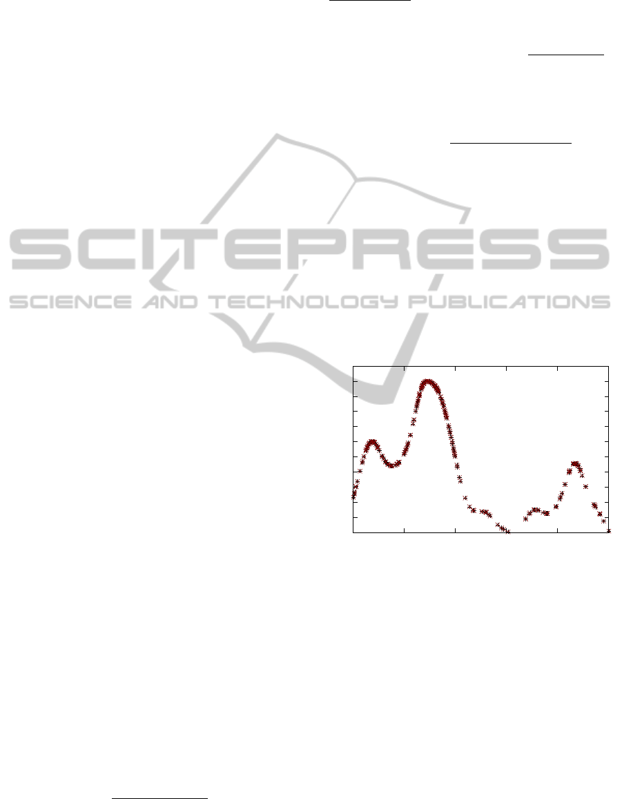
The density function of ASCDD can be consid-
ered as a distribution function, which describes the
distribution smoothly. The characters of clusters are
shown through the density evidently, namely the clus-
ter center has higher density than objects at edge, and
therefore the position and size of the clusters can be
indicated easily. Another important feature is that the
algorithm can be executed in any subspace, which is
simple and convenient for clustering particular sub-
space. Figure 1 shows an example of density for one
5
10
15
20
25
30
35
40
45
50
55
60
0 0.2 0.4 0.6 0.8 1
Density
Position of the objects
Figure 1: An example of density function.
dimensional subspace. The peaks are possible centers
of clusters, which are the key targets of our study.
3.1 Distance-density Threshold
Clustering is the next step after the density values are
calculated. The objects in a cluster are considered as
“connected” or “neighbors”. A threshold for choos-
ing proper neighbors called DDT (Distance-Density
Threshold) is introduced in ASCDD and is important
to the clustering step. The neighbors of an object o
i
are defined as follows:
Neighbor(o
i
) = {o
j
| d
e
A
o
i
,o
j
> DDT } (3)
DATA2013-2ndInternationalConferenceonDataManagementTechnologiesandApplications
16
An object and its neighbors are considered in the same
cluster.
Choosing a proper DDT is important, because
DDT can affect the size of clusters. Only the neigh-
bors with distance-density to the center object higher
than DDT meet the condition. It is apparent that the
larger DDT is chosen, the fewer neighbors will be se-
lected. Since d
e
A
o
i
,o
j
has a value between 0 and 1, the
parameter DDT has also to be determined within the
range (0,1). However, an improper DDT (too small
or a too big) can cause that all objects belong to one
cluster or there is no cluster. So a proper value for
DDT should be found in (0, 1) .
We notice these two values T
e
A
min
=
min
∀i
max
∀ j
(d
e
A
o
i
,o
j
)
and T
e
A
max
= max
∀i
max
∀ j
(d
e
A
o
i
,o
j
)
are important for the determination of DDT .
max
∀ j
(d
e
A
o
i
,o
j
) is the maximum distance-density of
o
i
with regard to the subspace
e
A. Each object o
i
has its maximum distance-density value with an
object o
j
in
e
A. Obviously, o
j
has the minimum Eu-
clidean distance to o
i
. T
e
A
min
is the smallest maximum
distance-density of all objects, and T
e
A
max
is the largest
distance-density of all objects. If DDT ≥ T
e
A
max
,
there will be no cluster result, because no object
has a neighbor. If DDT < T
e
A
min
, then all objects
will be clustered as one cluster, since all objects are
connected through the neighborhood. Obviously,
DDT should be set between T
e
A
min
and T
e
A
max
to get a
clustering result so DDT is defined as follows:
DDT = q · T
e
A
min
+ (1 − q) · T
e
A
max
, 0 < q < 1 (4)
Figure 2 illustrates an example of values T
e
A
min
and
T
e
A
max
. We notice that DDT should near T
e
A
min
for getting
a complete result. In Figure 2, o
min
is the object with
o
i
: o
1
o
2
o
3
o
min
· · · o
max
max
∀j
(d
eA
o
i
,o
j
)
T
eA
max
T
eA
min
Figure 2: An example of T
e
A
min
and T
e
A
max
.
distance-density T
e
A
min
, if DDT is close to T
e
A
min
, many
objects with distance-density values bigger than mini-
mum have the chances to be clustered in the next step.
Conversely, if DDT is close to T
e
A
max
, the amount of se-
lected objects will be much smaller. So by setting q
close to 1, ASCDD can get a relative complete result
in most cases.
Notice that T
e
A
min
and T
e
A
max
are different according
to
e
A, so DDT has normally also different values in
diverse
e
A.
3.2 Applying Entropy for Finding
Potential Subspace
Another issue is choosing the potential subspace with
clusters. Our solution is to apply entropy on detecting
subspaces. The authors of ENCLUS (Cheng et al.,
1999) introduced a method of applying entropy for
subspace clustering. However, ASCDD calculates
and applies entropy in subspace clustering with a dif-
ferent way.
Entropy is a measure of the amount of uncer-
tainty regarding a random variable. For a discrete
random variable X with n possible outcomes {x
i
:
i = 1, ··· ,n}, the Shannon entropy is defined as fol-
lows: H(X) = −
∑
n
∀i=1
p(x
i
) log p(x
i
), where p(·) is
the probability mass function. Obviously H(X) > 0.
Entropy has an important property, that the variables
with more uncertainty have lower entropy than the
variables with less uncertainty. For the clustering pur-
pose, we can say that a subspace with many clusters
has a low entropy.
The entropy reaches maximum if all outcomes are
equal.
H(p
1
,·· · , p
n
) ≤ H(
1
n
,·· · ,
1
n
) = −
n
∑
i=1
1
n
log
1
n
= log n
Sometimes normalized entropy is much more con-
venient, because it has a range [0, 1] for any n. The
normalized entropy is then defined as follows:
E(X) =
H(X)
logn
= −
n
∑
∀i=1
p(x
i
) log p(x
i
)/log n
Unlike ENCLUS we apply the probability of an
object o
i
in
e
A with
p(o
i
) =
D
e
A
o
i
∑
∀i
D
e
A
o
i
Obviously 0 ≤ p(o
i
) ≤ 1, and
∑
∀i
p(o
i
) = 1, the
o
i
with high density has also a big value p(o
i
), which
corresponds to the property of probability mass func-
tion.
SubspaceClusteringwithDistance-densityFunctionandEntropyinHigh-dimensionalData
17
We apply the normalized entropy E(
e
A) in AS-
CDD in order to facilitate the measurement and com-
parison of entropy values for any subspace. As intro-
duced above, E(
e
A) is defined as follows:
E(
e
A) = −
n
∑
∀i=1
p(o
i
) log p(o
i
)/log n
The E(
e
A) is applicable for any subspace
e
A. A
small E(
e
A) value indicates more uncertainties in
e
A,
which means there is more chance to detect clusters in
e
A. A big E(
e
A) shows that the objects distribute more
uniformly. The maximum value of E(
e
A) should be 1.
However, the objects with uniform distribution do not
have the same density values in ASCDD, because the
densities of objects in the middle are little bigger than
the densities at edge, but the difference is not large, so
in this situation E(
e
A) is smaller than 1 but very close
to 1.
The entropy of low dimensional subspace and
high dimensional subspace has some relations, which
helps us to speculate about the potential subspaces. If
the entropy of a subspace
e
A and a higher dimensional
subspace
e
A ∪ {a
i
} have a relation E(
e
A ∪ {a
i
}) <
E(
e
A), then the subspace
e
A ∪ {a
i
} has more clearly
separated clusters than
e
A. Conversely, if E(
e
A ∪
{a
i
}) > E(
e
A) it is likely that the subspace
e
A ∪ {a
i
}
has more uniform objects than the ones in the
e
A.
Our aim is exploring potential subspaces through
the property of entropy in order to reduce the com-
plexity. The exploring of high-dimensional potential
subspace from low-dimensional subspace uses this
principle: If E(
e
A ∪ {a
i
}) is not bigger than the en-
tropy of any subspace of
e
A ∪ {a
i
}, we say subspace a
i
can be integrated to subspace
e
A, which is described
as follows.
E(
e
A ∪{a
i
}) ≤ min({E(X) |∀X ∈
e
A ∪{a
i
}})
The process of searching potential subspaces
starts from one-dimensional subspace with low en-
tropy, for instance, a
1
is a subspace candidate, if the
entropy E(a
1
,a
2
) < min(E(a
1
),E(a
2
)) then the sub-
space candidate will expand from a
1
to the new sub-
space {a
1
,a
2
}. Suppose a subspace candidate
e
A sat-
isfies the condition: ∀a
i
, E(
e
A) < E(
e
A ∪ {a
i
}), then
e
A reaches its maximum dimension. The expansion
stops when the subspace candidate reaches the maxi-
mum dimension.
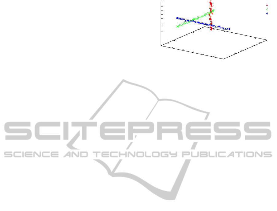
Figure 3 is a simple example for subspace cluster-
ing. It is not straightforward to cluster directly in the
three dimensional space, but if the objects are pro-
jected into any two dimensional subspace the clus-
tering process will be more effective because in each
-1
0
1
2
3
4
5
-1
0
1
2
3
4
5
6
-1
0
1
2
3
4
5
6
z
cluster 1
cluster 2
cluster 3
x
y
z
Figure 3: An example of three dimensional subspace clus-
tering.
two dimensional subspace one cluster is much tighter
than the other two clusters. Obviously, the two di-
mensional subspaces {x,y}, {y,z}, {x, z} are subspace
candidates. This result can also be verified through
the subspace searching method. The entropy of dif-
ferent subspaces has relations as the follows:
E(x, y);E(y,z);E(x,z) < E(x);E(y); E(z) < E(x, y, z)
The entropy of two dimensional subspace is smaller
than the entropy of one or three dimensional sub-
space. So each two dimensional subspace reaches the
maximum dimension. The subspace searching pro-
cess starts from one dimension and stops at two di-
mensional subspace, whereas the three dimensional
space will not be considered because it has a bigger
entropy value than two dimensional subspaces.
3.3 Algorithm
The clustering process of ASCDD consists of two
steps. The first step is searching the potential sub-
spaces and the second step is exploring clusters from
the potential subspaces.
We use greedy strategy to search the potential sub-
space, which is shown in Algorithm 1.
Searching the potential subspaces starts from one-
dimensional subspace with low entropy. A high-
dimensional subspace is considered as a subspace
candidate only with the principle that it has a lower
entropy than all its subspaces.
Algorithm 2 illustrates the clustering process of
ASCDD. The clustering process for a subspace can-
didate
e
A is divided into four steps.
I. ∀i, calculate D
e
A
o
i
.
II. Take the starting object o
s
that has the maximum
density of current set of objects O
current
.
III. Find all neighbors from o
s
, and set them as a
cluster S, then expand S by finding new neigh-
bors of objects in S until no new neighbor is
found.
DATA2013-2ndInternationalConferenceonDataManagementTechnologiesandApplications
18
Algorithm 1: Searching subspace.
Input: (A,O)
Output: Subspace Candidate Set: SCS
1 ascending sort E(a
i
): E(a
i
) ≤ E(a
j
) when i < j
2 SCS =
/
0
3 for i = 1 to |A| do
4 C = {a
i
}
5 for j = i + 1 to |A | do
6 minEntropy = min(E(C ),E(a
j
))
7 if E(C ∪ {a
j
}) <minEntropy then
8 C = C ∪ {a
j
}
9 SCS = SCS ∪{C }
Algorithm 2: Clustering.
Input: (A,O),SubspaceCandidateSet
Output: Set of all clusters
ˆ
S
1
ˆ
S =
/
0
2 foreach
e
A ⊆ SubspaceCandidateSet do
3 O
current
= O
4 ∀i, calculate D
e
A
o
i
5 while O
current
6=
/
0 do
6 o
s
has max(D
e
A
o
i
), ∀o
i
∈ O
current
7
e
O = Neighbor(o
s
)
8 Iteration: ∀o
i
∈
e
O, Neighbor(o
i
) ⊆
e
O
9 O
current
= O
current
−
e
O
10 S = (
e
A,
e
O),
ˆ
S =
ˆ
S ∪ S
IV. Remove objects in S from O
current
, repeat step II
until no more new cluster is found.
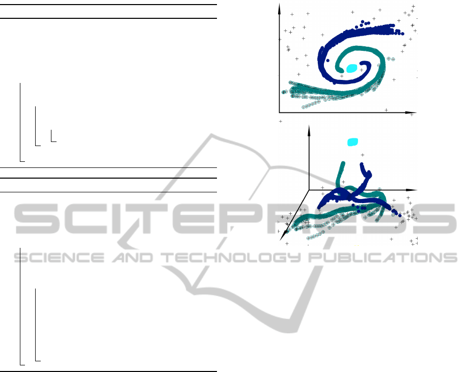
ASCDD could find arbitrary (convex or concave)
shaped clusters through extending the neighborhood.
For example, a cluster with a concave form is found as
follows: ASCDD may find an object with the highest
density in the cluster as the center object. Then the
process of searching and adding the new neighbors
to this cluster connects the objects together to reach
its original concave shape. The object with highest
density in a cluster is chosen as the “center” object.
However, this “center” object is possibly not the ge-
ometric center of the cluster. Figure 4 shows an ex-
ample of two-dimensional clustered objects (marked
with different colors) and corresponding density val-
ues of the objects. In this example, some center ob-
jects are at edges of the clusters. The objects in one
cluster are all the extensions of neighborhoods from
its center object.
The clusters are detected according to the order of
density values of center objects one by one (from the
highest density to the lowest density), which does not
Figure 4: Two-dimensional clustered objects & Three-
dimensional view of objects density.
depend on the input order of the objects. Therefore it
is not necessary to estimate the quantity of clusters in
ASCDD.
The time complexity of ASCDD depends on the
numbers of objects |O| and dimensions |A| and sub-
space candidates |SCS|. The run-time of density cal-
culation is O(|O|
2
) and the run-time of searching sub-
space depends on the subspace candidates, which can
between O(|S C S |) and O(2
|A|
).
4 EMPIRICAL EXPERIMENTS
A set of experiments was performed to observe the ef-
fectiveness and efficiency of ASCDD, particularly, fo-
cusing on the accuracy and run-time of clustering for
large quantities of data on high-dimensional spaces
and the ability for searching subspaces. All experi-
ments were carried out on a PC with 800MHz dual-
core processor, 4GB RAM, Linux operating system
and Java environment.
4.1 Synthetic Data
Firstly, we use synthetic data as experimental data
in order to make the experiment controllable and to
measure the accuracy easily. The data sets consist
of 10000 objects and 100 dimensions. 20 simulated
clusters are hidden in 10 different subspaces. The
clusters have different forms, e.g. convex and con-
SubspaceClusteringwithDistance-densityFunctionandEntropyinHigh-dimensionalData
19
cave forms. The subspaces without clusters are filled
with random objects.
We compare the results of ASCDD with differ-
ent settings of the parameter DDT . As we discussed
above, DDT depends on q, which is defined in Equa-
tion 4. So the problem of determining the DDT is
transformed to choose a q ∈ (0,1). Because the two
extreme situations q = 0 and q = 1 cause two results
respectively: no cluster object and all objects belong
to one cluster. When q is close to 1, almost all clus-
ter centers are taken into account by ASCDD, and
the clustering result is more complete than the re-
sults with a small q; When q approximates to 0, some
small clusters disappear, and the big clusters shrink
to small ones. However, the computation time will
be reduced with a small q. Generally speaking, alter-
ing q between 1 and 0 could adjust between details
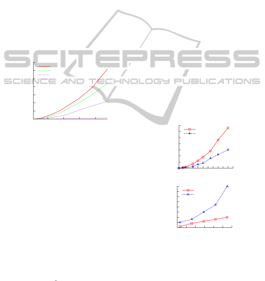
of clusters and run-time. Figure 5 presents the run-
0
5000
10000
15000
20000
25000
30000
35000
2 4 6 8
Time (seconds)
Number of objects
q=0.99
q=0.6
q=0.4
q=0.1
Figure 5: Run-time with different q.
time with four arbitrarily chosen q values. It is worth
mentioning that the clustering results do not change
much in a small range of q. In order to acquire com-
plete clustering results, we choose q = 0.96 in the fol-
lowing experiments, where 0.96 is just a discretionary
choice close to 1. Nevertheless, q can also be another
value ∈ (0.95,0.98) because the clustering results are
almost equal.
Since ENCLUS is one of the most famous sub-
space clustering method applying entropy, we com-
pare ASCDD with ENCLUS in the next experiment
with regard to potential subspaces and clustering re-
sults. ASCDD starts searching with the subspace with
lowest entropy, and expands the subspace in higher
dimensions by calculating and comparing the entropy
values. Finally all expected subspaces are obtained
correctly. We apply ENCLUS by setting the number
of units to 285 in order to keep averagely 35 objects in
each cell as the authors suggest. ENCLUS uses “en-
tropy < ω” and “interest
gain > ε” as the thresholds
for detecting subspace candidates. However, choos-
ing proper values for these two parameters is a chal-
lenge. We choose ω = 8.5, ε = 1 as described in the
article. ENCLUS does not find all the same subspace
candidates as ASCDD, ENCLUS finds a part of ex-
pected subspaces and many non-expected subspaces,
where no clusters exist. Even by altering the two
parameters with different combinations in ENCLUS,
the results of subspace candidates are still mixed with
non-expected subspaces.
Next we compare the clustering results between
ASCDD and ENCLUS. In this step ASCDD finds
the defined clusters in both convex and concave
forms with high precision. ENCLUS uses grid-based
method by searching the clusters firstly through the
grids in one dimensional subspace, and combines the
clusters in high-dimensional subspace to search more
clusters. In this experiment the result of ENCLUS
includes just some simple convex clusters correctly.
Some concave clusters are bound together as one clus-
ter and some are separated to small clusters. Unlike
ENCLUS, who has to search each low-dimensional
subspace of a subspace candidate, ASCDD can di-
rectly focus on the subspace candidates for searching
clusters.
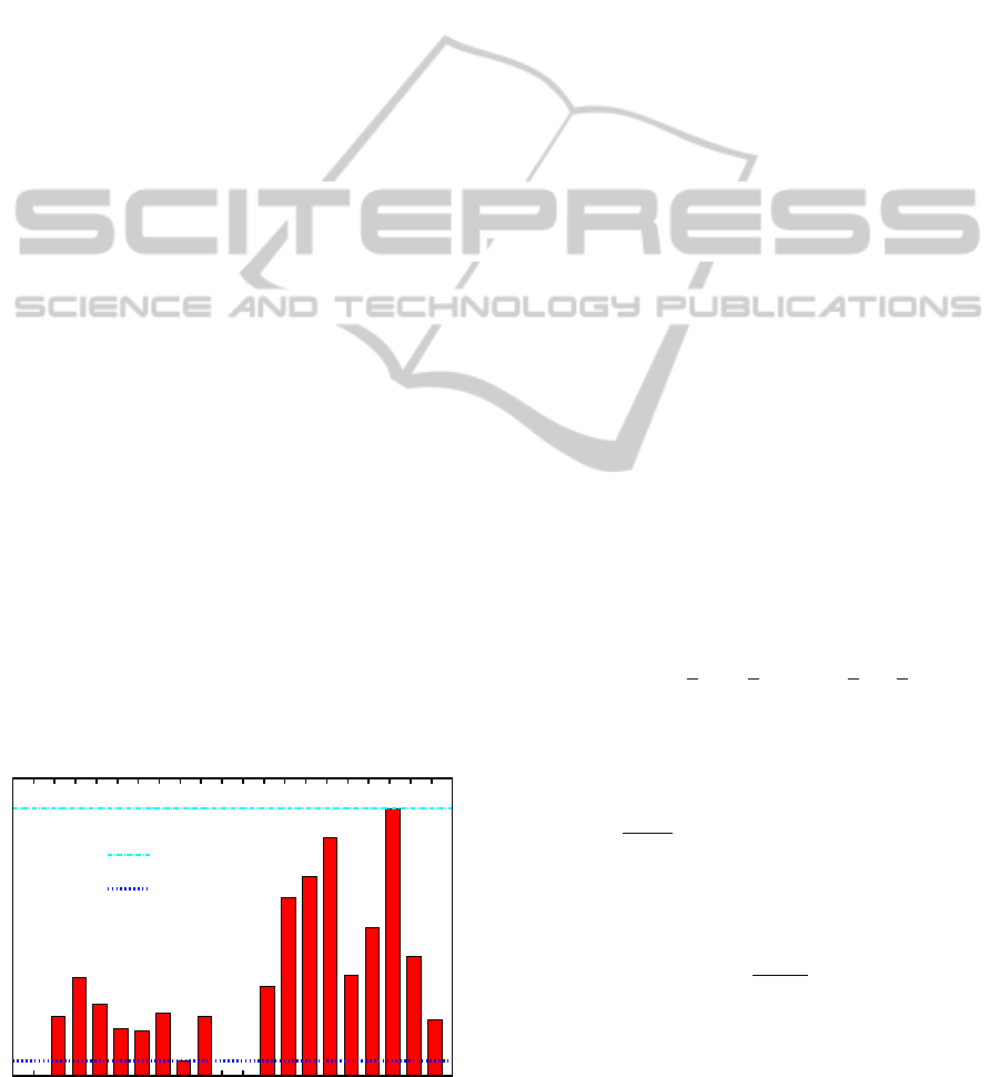
The efficiency evaluation of ASCDD and EN-
CLUS are illustrated in Figure 6. This evaluation is
based on subsets of the synthetic data set. ASCDD
and ENCLUS use the same parameter settings as in
the former experiment.
0
5000
10000
15000
20000
25000
30000
35000
1 2 3 4 5 6 7 8 9
(x10
3
)
Time (seconds)
(a) Number of objects
ASCDD
ENCLUS
0
500
1000
1500
2000
2500
3000
3500
4000
10 20 30 40 50 60 70
Time (seconds)
(b) Number of dimensions
ASCDD
ENCLUS
Figure 6: Run-time compared with ENCLUS.
ASCDD scales very well with an increasing di-
mensionality. As we can see, the run-time of ASCDD
increases linearly if the number of dimensions grows.
The reason is that ASCDD searches firstly only the
subspace candidates, and the clustering process ex-
ecutes directly on high dimensional subspace candi-
dates. ASCDD has almost the same run-time for a
DATA2013-2ndInternationalConferenceonDataManagementTechnologiesandApplications
20
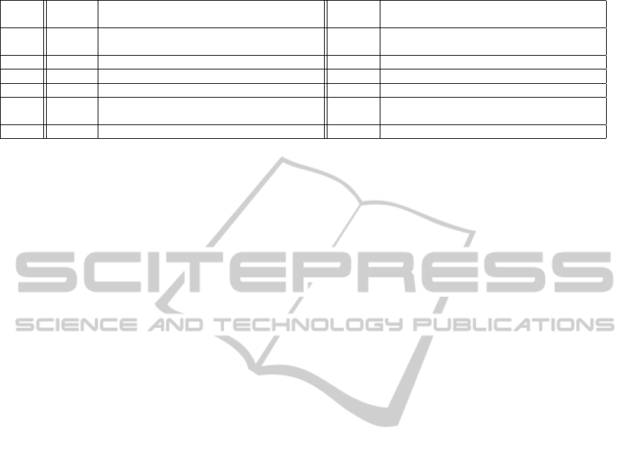
Table 1: Results of ASCDD and ENCLUS on “Gas Sensor Array Drift”.
Cluster ASCDD ENCLUS
Accuracy Subspace Accuracy Subspace
1 68% 76, 113, 17, 4, 79, 70, 14, 68, 121, 57, 15, 6, 7, 53, 118,
12, 54, 62, 127
41% 113, 4, 79, 70, 68, 57, 15, 54, 7, 14, 53, 118, 83, 14, 73
2 67% 15, 6, 78, 49, 7, 12, 55, 63 55% 20, 6, 78, 30, 19, 7, 66, 23, 11, 50, 93
3 39% 47, 24, 107, 111, 88, 97, 99, 105 31% 88, 40, 26, 113, 105, 95, 33, 28, 16
4 68% 44, 108, 39, 47, 24, 103, 111, 88, 97, 99, 105 52% 111, 23, 108, 75, 39, 94, 47, 85
5 34% 112, 56, 120, 122, 98, 16, 35, 106, 43, 80, 36, 108, 24,
107, 88, 97, 99, 105
19% 112, 43, 106, 16, 80, 24, 74, 87, 86, 98, 19, 108, 58
6 88% 65, 9, 76, 4, 79, 70, 14, 68, 15, 6, 78, 7, 12, 39, 47, 103 59% 65, 83, 4, 68, 70, 6, 81, 14, 7, 103, 79
clustering within a subspace with no matter high or
low dimension.
With increasing number of objects the run-time
of ASCDD grows quadratically, which is longer than
ENCLUS in this situation. The reason is that the cal-
culation of density for one object in ASCDD involves
all objects and ENCLUS works similar to CLIQUE
that separates the objects into grids, which is not sen-
sitive to amount of objects. Although the scalability
of ASCDD related to the size of objects is not linear,
the complexity ensures getting a complete clustering
result. Of course the run-time with regard to the num-
ber of objects depends also on the parameter setting
because choosing a DDT that yields many objects in
the clustering result takes more time than with a DDT
that involves fewer objects.
ENCLUS finds almost the same low dimensional
subspace candidates, but ENCLUS is slower than AS-
CDD for high dimensional subspace, because EN-
CLUS does clustering only from low to high dimen-
sional subspace, which takes much time than direct
clustering in high dimensional subspace as ASCDD.
4.2 Real Data
The data set “Gas Sensor Array Drift” has been ob-
tained from the UC Irvine Machine Learning Repos-
itory (Frank and Asuncion, 2010). This data set cor-
responds to the measurements of 16 chemical sensors
utilized in simulations for drift compensation in dis-
criminating six gas types (Ammonia, Acetaldehyde,
Acetone, Ethylene, Ethanol, and Toluene) at various
concentrations. The data is prepared for the chemo-
sensor research community and artificial intelligence
to develop strategies to cope with sensor/concept
drift. The dataset contains 128 dimensions, 13910
measurements with six clusters (six gas types), we
applied ASCDD and ENCLUS on the data without
cluster labels, the results were then compared with
the cluster labels. The clusters are located in differ-
ent subspaces, which means the particular subspaces
can specialize detecting the gas types. We illustrate
some examples of the clustering result and the accu-
racies of data related to months one and two in Table
1. The accuracy is defined as the proportion of the
number of correctly clustered objects to the number
of objects in that cluster.
This clustering process takes 1440 seconds with
ASCDD and 4410 seconds with ENCLUS. Compared
with ENCLUS, ASCDD is more efficient on high-
dimensional subspace and is able to detect the clusters
directly on these subspaces with higher precision.
5 CONCLUSIONS
Departing from the traditional clustering methods,
ASCDD is suitable for complex data with arbitrary
forms. It provides useful distribution information and
can be applied easily with just one simple parameter
DDT by clustering. The clusters are detected accord-
ing to their densities, which does not depend on the in-
put order. The results of ASCDD in our experiments
show high accuracy.
In this paper we improve the methods of sub-
space detection and parameter determination in
the subspace clustering method ASCDD for high-
dimensional data set. By adhibiting entropy, ASCDD
is able to detect high-dimensional subspace candi-
dates easily, where a subspace with low entropy is
considered as a potential subspace. We develop a way
to detect subspace candidates to reach its maximum
dimensions. ASCDD can directly find clusters within
the located subspace candidates. Since the cluster-
ing result and quality depend on choosing the param-
eter DDT , we investigate the DDT and introduce a
method of choosing this parameter. The DDT can be
chosen in accordance with the tendencies to complete
clustering results or short run-time. One of our future
works will be reducing the calculation time with very
high number of objects.
REFERENCES
Aggarwal, C. C., Wolf, J. L., Yu, P. S., Procopiuc, C., and
Park, J. S. (1999). Fast algorithms for projected clus-
SubspaceClusteringwithDistance-densityFunctionandEntropyinHigh-dimensionalData
21

tering. In Proceedings of the 1999 ACM SIGMOD in-
ternational conference on Management of data, SIG-
MOD ’99, pages 61–72. ACM.
Aggarwal, C. C. and Yu, P. S. (2000). Finding general-
ized projected clusters in high dimensional spaces. In
Proceedings of the 2000 ACM SIGMOD international
conference on Management of data, SIGMOD ’00,
pages 70–81. ACM.
Agrawal, R., Gehrke, J., Gunopulos, D., and Raghavan, P.
(1998). Automatic subspace clustering of high dimen-
sional data for data mining applications. In Proceed-
ings of the 1998 ACM SIGMOD international confer-
ence on Management of data, SIGMOD ’98, pages
94–105. ACM.
Chang, J.-W. and Jin, D.-S. (2002). A new cell-based clus-
tering method for large, high-dimensional data in data
mining applications. In Proceedings of the 2002 ACM
symposium on Applied computing, SAC ’02, pages
503–507. ACM.
Cheng, C.-H., Fu, A. W., and Zhang, Y. (1999). Entropy-
based subspace clustering for mining numerical data.
In Proceedings of the fifth ACM SIGKDD interna-
tional conference on Knowledge discovery and data
mining, KDD ’99, pages 84–93. ACM.
Ester, M., Kriegel, H.-P., Sander, J., and Xu, X. (1996).
A density-based algorithm for discovering clusters in
large spatial databases with noise. In Proceedings of
the 2nd International Conference on Knowledge Dis-
covery and Data mining, volume 1996, pages 226–
231. AAAI Press.
Frank, A. and Asuncion, A. (2010). UCI machine learning
repository.
Friedman, J. H. and Meulman, J. J. (2004). Clustering ob-
jects on subsets of attributes. Journal of the Royal Sta-
tistical Society: Series B (Statistical Methodology),
pages 815–849.
Goil, S., Nagesh, H., and Choudhary, A. (1999). Mafia:
Efficient and scalable subspace clustering for very
large data sets. Technical Report CPDC-TR-9906-
010, Northwestern University.
Hinneburg, A. and Gabriel, H.-H. (2007). Denclue 2.0: fast
clustering based on kernel density estimation. In Pro-
ceedings of the 7th international conference on Intel-
ligent data analysis, IDA’07, pages 70–80. Springer-
Verlag.
Hinneburg, A., Hinneburg, E., and Keim, D. A. (1998).
An efficient approach to clustering in large multime-
dia databases with noise. In Proc. 4rd Int. Conf. on
Knowledge Discovery and Data Mining, pages 58–65.
AAAI Press.
Kriegel, H.-P., Kr
¨
oger, P., and Zimek, A. (2009). Clustering
high-dimensional data: A survey on subspace cluster-
ing, pattern-based clustering, and correlation cluster-
ing. ACM Transactions on Knowledge Discovery from
Data, 3:1:1–1:58.
Kr
¨
oger, P., Kriegel, H.-P., and Kailing, K. (2004). Density-
connected subspace clustering for high-dimensional
data. In Proc. SIAM Int. Conf. on Data Mining
(SDM’04), pages 246–257.
MacQueen, J. B. (1967). Some methods for classification
and analysis of multivariate observations. In Proc. of
the fifth Berkeley Symposium on Mathematical Statis-
tics and Probability, volume 1, pages 281–297. Uni-
versity of California Press.
M
¨
uller, E., G
¨
unnemann, S., Assent, I., and Seidl, T. (2009).
Evaluating clustering in subspace projections of high
dimensional data. Proceedings of the VLDB Endow-
ment, 2(1):1270–1281.
Parsons, L., Haque, E., and Liu, H. (2004). Subspace clus-
tering for high dimensional data: A review. SIGKDD
Explor. Newsl., 6:90–105.
Procopiuc, C. M., Jones, M., Agarwal, P. K., and Murali,
T. M. (2002). A monte carlo algorithm for fast pro-
jective clustering. In Proceedings of the 2002 ACM
SIGMOD international conference on Management of
data, SIGMOD ’02, pages 418–427. ACM.
Sim, K., Gopalkrishnan, V., Zimek, A., and Cong, G.
(2012). A survey on enhanced subspace clustering.
Data Mining and Knowledge Discovery, pages 1–66.
Woo, K.-G., Lee, J.-H., Kim, M.-H., and Lee, Y.-J. (2004).
Findit: a fast and intelligent subspace clustering algo-
rithm using dimension voting. Information and Soft-
ware Technology, 46(4):255–271.
Zhao, J. and Conrad, S. (2012). Automatic subspace clus-
tering with density function. In International Confen-
rence on Data Technologies and Applications, DATA
2012, pages 63–69. SciTePress Digital Library.
DATA2013-2ndInternationalConferenceonDataManagementTechnologiesandApplications
22
