Modulation-mode and Power Assignment

in SVD-assisted MIMO Systems

with Transmitter-side Antennas Correlation

Andreas Ahrens

, Francisco Cano-Broncano

and C´esar Benavente-Peces

Hochschule Wismar, University of Technology, Business and Design, Philipp-M¨uller-Straße 14, 23966 Wismar, Germany

Universidad Polit´ecnica de Madrid, Ctra. Valencia. km. 7, 28031 Madrid, Spain

Keywords:

Multiple-Input Multiple-Output System, Singular-Value Decomposition, Bit Allocation, Power Allocation,

Antennas Correlation, Wireless Transmission.

Abstract:

Multiple-input multiple-output (MIMO) systems can provide a noticeable improvement in channel perfor-

mance. Nevertheless some perturbances affect the capability of this technique to get the expected improve-

ment. Due to the use of multiple antennas at the same front-end and their close spacing the so called antennas

correlation effect appears. Antennas correlation can drastically affect the channel behaviour by increasing the

bit-error rate (BER) and dropping its capability. This paper analyses the impact of transmitter-side antennas

correlation on the MIMO system performance. The singular value decomposition (SVD) is used to transform

the MIMO channel into independent layers. Afterwards bit and power allocation techniques are applied in

order to obtain the best performance.

1 INTRODUCTION

MIMO communication systems have been studied

along the last two decades and incorporated in com-

munication standards due to their ability of increasing

the channel capabilities (lower bit-error rate (BER)

and larger data rates) without requiring additional

transmit power and bandwidth. In order to obtain the

full advantages promised by MIMO techniques, addi-

tional signal processing should be applied. Singular-

value decomposition (SVD) is a popular techniques

which allows removing the inter-antenna interfer-

ences due to the multiple antennas arrangements both

at the transmitter and the receiver sides (Haykin,

2002). The SVD transforms the MIMO channel

into multiple independent layers (single-input single-

output channels, SISO). In order to get the full ben-

eﬁts of using the SVD, perfect channel state infor-

mation should be available both at the transmit and

receive front-ends. Once the SVD has been applied

each layer is characterized by a singular value (gain

factor). The ideal set-up is that in which after SVD

all the layers behave in the same way, that is, all the

singular values take the same value. Usually this sit-

uation does not take place and layers have different

performances. MIMO systems beneﬁt from scattered

environments where multipath is present and take ad-

vantage of the multipath effect by using signal pro-

cessing techniques (as the aforementioned singular-

value decomposition) (K¨uhn, 2006).

MIMO wireless channels are affected by the vari-

ous disturbances inﬂuencing regular wireless commu-

nication systems. Additionally, due to the use of mul-

tiple antennas at both the transmit and receive sides,

and the typical close spacing of the antennas due to

physical limitations, the so called antennas correla-

tion effect arises (Lee, 1973; Salz and Winters, 1994;

Shiu et al., 2000).

Therefore, MIMO scenarios with uncorrelated

channel coefﬁcients have reached a state of maturity.

By contrast, MIMO scenarios with correlated channel

coefﬁcients require substantial further research.

Antennas correlation diminishes multipath reach-

ness, essential to MIMO techniques. Due to that ef-

fect the various paths from each transmitter-side an-

tenna to each receiver-side antenna become similar.

Under this condition applying the SVD deals to sin-

gular values which are quite different and the ratio be-

tween the layers having largest and smallest singular

values becomes high. This means that predominant

layers arise, some with large singular values which

have a pretty good performance and others with quite

225

Ahrens A., Cano-Broncano F. and Benavente-Peces C..

Modulation-mode and Power Assignment in SVD-assisted MIMO Systems with Transmitter-side Antennas Correlation.

DOI: 10.5220/0004497102250232

In Proceedings of the 10th International Conference on Signal Processing and Multimedia Applications and 10th International Conference on Wireless

Information Networks and Systems (WINSYS-2013), pages 225-232

ISBN: 978-989-8565-74-7

 2013 SCITEPRESS (Science and Technology Publications, Lda.)

low singular values which have a poor performance.

In consequence this paper analyzes and charac-

terizes the antennas correlation effect focussing our

attention on the transmitter-side. The analysis re-

marks the parameters affecting the correlation effect

and their inﬂuence on the overallsystem performance.

Additional techniques can be applied to improve

the MIMO system performance. Some of these tech-

niques are bit and power allocation (Zhou et al., 2005;

Mutti and Dahlhaus, 2004). Based on the MIMO lay-

ers performance various transmission modes can be

deﬁned by allocating a different number of bits per

symbol along the various layers while maintaining the

overall data rate. Through the analysis of some exem-

plary transmission modes this paper shows that not

all the layers should be activated in order to obtain

the best results.

Power allocation techniques distribute the trans-

mit available power along the different transmit an-

tennas. One of the most popular techniques is the so

called water-ﬁlling. Based on the layers quality it is

determined the layers which should be activated and

hence the total available transmit power is appropri-

ately distributed.

Against this background, the novel contribution of

this paper is that we demonstrate the beneﬁts of amal-

gamating a suitable choice of activated MIMO layers

and number of bits per symbol together with the ap-

propriate allocation of the transmit power under the

constraint of a given ﬁxed data throughput. Our re-

sults showthat under the constraint of correlation only

a few layer should be used for the data transmission

when minimizing the overall bit-error rate.

The remaining part of this paper is organized as

follows. Section 2 describes the MIMO system model

including the antennas correlation characterization.

The bit- and power assignment in correlated channel

situation is discussed in section 3. The obtained re-

sults are presented and interpreted in section 4. Fi-

nally section 5 remarks the main results obtained in

this investigation.

2 MIMO SYSTEM MODEL

This section is aimed to establish the MIMO system

model affected by transmitter-side antennas correla-

tion effect. First, the correlation coefﬁcients are de-

ﬁned and characterized in order to ﬁnally describe the

overall MIMO system model.

2.1 Transmitter-side Correlation

Coefﬁcients Characterization

The correlation effect is described by the correla-

tion coefﬁcients. Transmitter-side antennas correla-

tion coefﬁcients describe the similitude between paths

corresponding to a pair of antennas (at the transmit-

ter side) with respect to a reference antenna (at the

receiver side). Fig. 1 describes the basic set-up for

obtaining the correlation coefﬁcient, where d is the

transmitter-side antennas spacing, d

is the distance

between transmit antenna #1 and the receiver-side an-

tenna (taken as reference) and d

is the distance from

transmit antenna #2 to the reference receive antenna

(it is assumed d << d

); φ is the departure an-

gle. In consequence two paths are described and the

correlation coefﬁcient describes how like they are.

When analyzing the system conﬁguration, presented

d/2

antenna #1

Transmitter side

Receiver side

antenna #1

antenna #2

Figure 1: Antennas’ physical disposition: two transmit and

one receive antennas.

in Fig. 1, the correlation between the signal s

(t), i. e.

the signal arriving at the receive antenna from trans-

mit antenna #1, and the signal s

(t), i. e. the signal

arriving at the receive antenna from transmit antenna

#2, is given by

(TX)

1,2

E{s

(t) ·s

∗

(t)}−E{s

(t)}·E{s

(t)}

E{s

(t) ·s

∗

(t)}·

E{s

(t) ·s

∗

(t)}

(1)

and simpliﬁes as shown in (Cano-Broncano et al.,

2013) to

(TX)

1,2

= e

−j2π

−d

)

. (2)

The transmit antenna separation d

= d/λ given in

wavelengths units can be expressed as

−d

= d

·cos(φ) . (3)

Inserting (3) in (2), the transmitter-side correlation

coefﬁcient is given by

(TX)

1,2

= e

j2πd

cos(φ)

. (4)

The antennas path correlation coefﬁcient for line of

sight (LOS) trajectories depends on the antennas sep-

aration d

and the transmit antennas reference axis

WINSYS2013-InternationalConferenceonWirelessInformationNetworksandSystems

226

0 1 2 3 4 5

0.2

0.4

0.6

0.8

|ρ

(TX)

1,2

(φ,σ

)| →

→

φ = 30

◦

φ = 60

◦

φ = 90

◦

Figure 2: Dependency of |ρ

(TX)

1,2

(φ,σ

)| as a function of σ

and φ assuming an antennas separation in wavelengths of

= 1/4.

0 5 10 15 20

0.2

0.4

0.6

0.8

|ρ

(TX)

1,2

(φ,σ

)| →

→

φ = 30

◦

φ = 60

◦

φ = 90

◦

Figure 3: Dependency of |ρ

(TX)

1,2

(φ,σ

)| as a function of σ

and φ assuming a wavelength speciﬁc antenna separation of

= 1/16.

rotation angle φ (or signals angle of departure). By

taking the scattered environment of wireless chan-

nels into consideration, the transmit antennas refer-

ence axis rotation angle φ becomes time-variant and

(4) results in:

(TX)

1,2

= E{e

j2πd

cos(φ+ξ

)

} . (5)

The parameter ξ

in (5) expresses the randomness of

the angles for the various scatters and is described by

a Gaussian distribution with zero mean and variance

. Calculating the expectation under this assumption

leads to the following equation:

(TX)

1,2

(φ,σ

) = e

j2πd

cos(φ)

−

(2πd

sin(φ)σ

)

. (6)

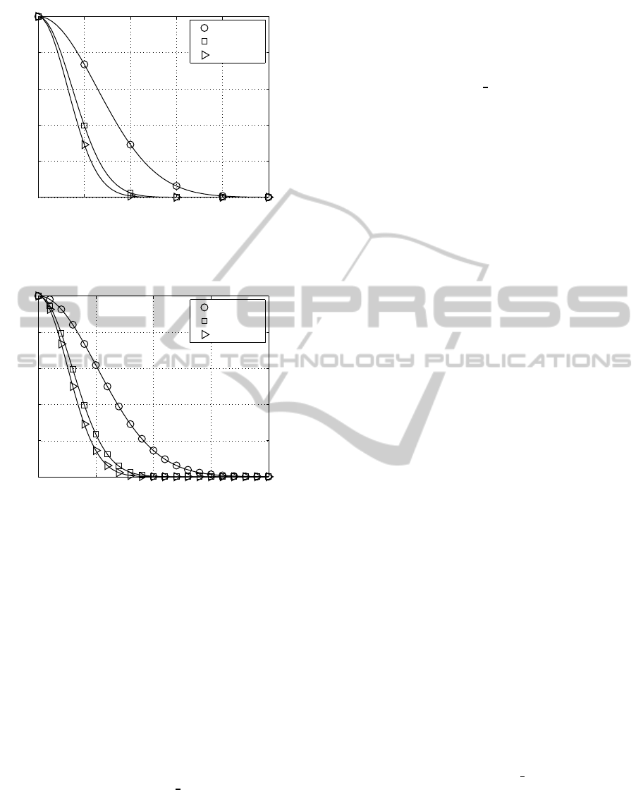
When analyzing Fig. 2 and Fig. 3, high coefﬁcients

correlation appears for small parameters of φ and σ

Additionally, in case of a small antenna separation,

i. e. reducing d

, the received signals s

(t) and s

(t)

become even more similar.

2.2 Correlated MIMO System Model

The (n

×n

) system matrix H of a correlated MIMO

system model is given by

vec(H) = R

·vec(G) (7)

where G is a (n

×n

) uncorrelated channel matrix

with independent, identically distributed complex-

valued Rayleigh elements and vec(·) is the opera-

tor stacking the matrix G into a vector column-wise

(Oestges, 2006). Based on the quite common assump-

tion that the correlation between the antenna elements

at the transmitter side is independent from the correla-

tion between the antenna elements at the receiverside,

the correlation matrix R

can be decomposed into a

transmitter side correlation matrix R

and a receiver

side correlation matrix R

following the Kronecker

product ⊗. Under this assumption the matrix R

formulated as

= R

⊗R

. (8)

In this paper, no correlation at the receiver side is as-

sumed. Therefore, the (n

×n

) receiver-side corre-

lation matrix R

simpliﬁes to

= I (9)

with the matrix I describing the identity matrix. The

×n

) correlation matrix R

for the investigated

(4×4) MIMO system is ﬁnally given by:

(4×4)







1 ρ

(TX)

1 ρ

(TX)

1 ρ

(TX)







(10)

Therein, the correlation coefﬁcient ρ

(TX)

k,ℓ

describes

the transmitter side correlation between the transmit

antenna k and ℓ. Taking line-of-sight conditions into

account, the correlation coefﬁcient results according

to (4) in

(TX)

k,ℓ

= e

−j2π(k−ℓ) d

cos(φ)

for k < ℓ . (11)

Extending these results to scattered conditions, the

transmitter side correlation coefﬁcient results accord-

ing to (5) for k < ℓ in

(TX)

k,ℓ

(φ,σ

) = e

−j2π(k−ℓ)d

cos(φ)

−

(2π(k−ℓ)d

sin(φ)σ

)

(12)

For the calculation of the transmitter-side correlation

coefﬁcient for values of k > ℓ it can be exploited that

the values of the correlation coefﬁcients are complex

conjugated. This is due to the sign change when com-

puting the distance difference between antennas with

Modulation-modeandPowerAssignmentinSVD-assistedMIMOSystemswithTransmitter-sideAntennasCorrelation

227

different antenna reference (see Fig. 4). Finally, the

following equation can be used to calculate the corre-

lation coefﬁcient for values of k > ℓ

(TX)

ℓ,k

= ρ

∗(TX)

k,ℓ

. (13)

d/2

antenna #2

antenna #3

antenna #1

antenna #4

Figure 4: Antennas’ physical disposition: four transmit and

one receive antennas.

Having frequency non-selective MIMO channels,

the whole MIMO system can be decomposed into a

number of independent, non-interfering layers. Us-

ing singular-value decomposition (SVD), the result-

ing system model is depicted in Fig. 5, where the

weighting factor

ℓ,k

represents the positive square

roots of the eigenvalues of the system matrix per

MIMO layer ℓ and per transmitted data block k. The

transmitted complex input symbol per MIMO layer

ℓ is described by c

ℓ,k

and the additive, white Gaus-

sian noise (AWGN) by w

ℓ,k

, respectively. In gen-

ℓ,k

Figure 5: Resulting system model per MIMO layer ℓ and

transmitted data block k.

eral, correlation inﬂuenced the unequal weighting of

the different layers. In order to carefully study the

inﬂuence of the correlation, two channel constella-

tions are chosen as highlighted in Tab. 1. The cor-

responding unequal weighting of the different lay-

ers is shown in Fig. 6 and Fig. 7 for an exemplarily

studied (4 ×4) MIMO system. Therein, the differ-

ence in the layer-speciﬁc ﬂuctuations is described by

the probability density function (pdf) of the parame-

ter ϑ =

ℓ=4,k

ℓ=1,k

, which shows the unequal

weighting of the different layers within the MIMO

system.

The ratio between the smallest and the largest sin-

gular values is an appropriate way to infer the anten-

Table 1: Parameters of the of the investigated channel con-

stellations.

Description φ σ

Weak correlation 30

◦

1 1

Strong correlation 30

◦

1 0,25

0 0.1 0.2 0.3 0.4 0.5

0.005

0.01

0.015

0.02

uncorrelated

correlated

pdf →

ϑ →

Figure 6: PDF (probability density function) of the ratio

ϑ between the smallest and the largest singular value for

weakly correlated (solid line) as well as uncorrelated (dot-

ted line) frequency non-selective (4 ×4) MIMO channels

= 1, φ = 30

◦

and σ

= 1,0).

0 0.1 0.2 0.3 0.4 0.5

0.005

0.01

0.015

0.02

uncorrelated

correlated

pdf →

ϑ →

Figure 7: PDF (probability density function) of the ratio

ϑ between the smallest and the largest singular value for

strongly correlated (solid line) as well as uncorrelated (dot-

ted line) frequency non-selective (4 ×4) MIMO channels

= 1/4, φ = 30

◦

and σ

= 1,0).

nas correlation effects. When this parameter ϑ ap-

proaches the unity the MIMO channel is close to the

best performance which is reached when all the layers

have the same performance (assuming the same noise

power at the receiver-side). In this particular case the

layer-speciﬁc weighting factors, i.e., the singular val-

ues, are very similar. For weak antennas correlation,

as depicted in Fig. 6, this parameter decreases which

means some layers performs better than others and the

WINSYS2013-InternationalConferenceonWirelessInformationNetworksandSystems

228

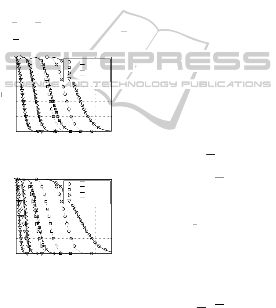
overall MIMO channel performance drops. When an-

tennas correlation is signiﬁcantly high, the parameter

ϑ becomes smaller, meaning a noticeable difference

in the performance of the various layer. Now, pre-

dominant strong and weak layers appear which de-

creases the overall channel performance (by increas-

ing the BER).

The distribution of the layer-speciﬁc characteris-

tic can be studied when analyzing the CCDF (com-

plementary cumulative distribution function) for the

different degrees of correlation as shown in Fig. 8 and

Fig. 9. The antennas correlation increases the prob-

ability of having layers with larger values (see lay-

ers

and

) and increases for weak layers the

probability of having lower values (see layers

and

0 1 2 3 4 5 6

0.2

0.4

0.6

0.8

(1st layer)

(2nd layer)

(3rd layer)

(4th layer)

Prob{

ℓ

≥U} →

U →

Figure 8: CCDF of the layer-speciﬁc distribution for weakly

correlated (solid line) as well as uncorrelated (dotted line)

frequency non-selective (4 ×4) MIMO channels (d

= 1,

φ = 30

◦

and σ

= 1,0).

0 1 2 3 4 5 6

0.2

0.4

0.6

0.8

(1st layer)

(2nd layer)

(3rd layer)

(4th layer)

Prob{

ℓ

≥U} →

U →

Figure 9: CCDF of the layer-speciﬁc distribution for

strongly correlated (solid line) as well as uncorrelated (dot-

ted line) frequency non-selective (4 ×4) MIMO channels

= 1/4, φ = 30

◦

and σ

= 1,0).

The inspection of the CCDF also provides rele-

vant information to predict the MIMO channel per-

formance. Increasing antennas correlation spreads the

singular values CCDF curves. For the non-correlated

case, the various layers CCDF seem to be more con-

centrated. In the ideal case all of them overlap and

the best performance is obtained. Weak correlation

spreads the curves by right shifting those correspond-

ing to the highest singular values increasing the prob-

ability of getting large values in contrast to the small-

est singular values. Under strong antennas correlation

the CCDF curve for the largest singular values are in-

deed more right shifted while the smallest ones are

left shifted. In consequence, in this case the probabil-

ity of the largest singular value to obtain a high value

increases while the probability of taking the smallest

singular values a lower value also increases dealing to

the MIMO channel worse performance.

3 BIT- AND POWER

ASSIGNMENT

Assuming M-ary Quadrature Amplitude Modulation

(QAM), the argument ρ = U

of the complemen-

tary error function (Kalet, 1987; Proakis, 2000) can

be used to optimize the quality of a data communi-

cation system by taking the half-vertical eye-opening

and the noise power per quadrature componentU

at the detector input into account (Ahrens and Lange,

2008). The half-vertical eye-opening per MIMO layer

ℓ and per transmitted symbol block k results in

(ℓ,k)

ℓ,k

·U

sℓ

, (14)

where U

sℓ

denotes the half-level transmit amplitude

assuming M

ℓ

-ary QAM and

ℓ,k

represents the pos-

itive square roots of the eigenvalues of the matrix

H. The average transmit power P

sℓ

per MIMO

layer ℓ determines the half-level transmit amplitude

sℓ

and is given by

sℓ

ℓ

−1) . (15)

Activating L ≤ min(n

) MIMO layers, the overall

transmit power P

∑

ℓ=1

sℓ

can be calculated.

Power Allocation (PA) can be used to balance the

BER in the different numbers of activated MIMO lay-

ers (Ahrens and Lange, 2008). The resulting layer-

speciﬁc system model including power allocation is

highlighted in Fig. 10. The layer-speciﬁc power allo-

cation factors

√

ℓ,k

adjust the half-vertical eye open-

ing according to

(ℓ,k)

APA

√

ℓ,k

·U

sℓ

. (16)

Modulation-modeandPowerAssignmentinSVD-assistedMIMOSystemswithTransmitter-sideAntennasCorrelation

229

replacements

ℓ,k

√

ℓ,k

Figure 10: Resulting layer-speciﬁc system model including

MIMO-layer PA.

This results in the layer-speciﬁc transmit power per

symbol block k

(ℓ,k)

sPA

= p

ℓ,k

sℓ

. (17)

Taking all activated MIMO layers into account, the

overall transmit power per symbol block k is obtained

(k)

sPA

∑

ℓ=1

(ℓ,k)

sPA

= P

. (18)

In order to balance the BER in the different numbers

of activated MIMO layers, solutions for the so far un-

known PA parameters are needed.

A simpliﬁed PA solution can be found when guar-

anteeing that the signal-to-noise-ratio at the detector

input is the same for all activated MIMO layers per

data block k. In this particular case, the following

condition should be ensured for the signal-to-noise ra-

tio at the detector input

(ℓ,k)



(ℓ,k)

APA



= constant ℓ = 1, 2,··· ,L .

(19)

When assuming an identical detector input noise vari-

ance U

for each channel output symbol the before-

hand introduces Equal-SNR criteria requires the same

half vertical eye opening of each channel output sym-

bol

(ℓ,k)

APA

= constant ℓ = 1, 2,··· ,L . (20)

The power to be allocated to each activated MIMO

layer ℓ and transmitted data block k can be shown to

be calculated as follows:

ℓ,k

sℓ

·ξ

ℓ,k

∑

ν=1

sν

·ξ

ν,k

(21)

and guarantees for each channel output symbol (ℓ =

1,··· ,L) the same half vertical eye opening of

(ℓ,k)

APA

√

ℓ,k

·U

sℓ

∑

ν=1

sν

ν,k

(22)

Together with the identical detector input noise vari-

ance for each channel output symbol, the above-

mentioned equal quality scenario is encountered.

Table 2: Investigated QAM transmission modes.

throughput layer 1 layer 2 layer 3 layer 4

8 bit/s/Hz 256 0 0 0

8 bit/s/Hz 64 4 0 0

8 bit/s/Hz 16 16 0 0

8 bit/s/Hz 16 4 4 0

8 bit/s/Hz 4 4 4 4

4 RESULTS

In this work a (4×4) MIMO system with transmitter-

side antennas correlation is studied.

In order to transmit at a ﬁxed data rate while

maintaining the best possible integrity, i. e., bit-error

rate, an appropriate number of MIMO layers has to

be used, which depends on the speciﬁc transmission

mode, as detailed in Tab. 1.

The choice of ﬁxed transmission modes regardless

of the channel quality can be justiﬁed when analyz-

ing the probability of choosing a speciﬁc transmis-

sion mode by using optimal bitloading (Wong et al.,

1999). As highlighted in Table 3 for uncorrelated

MIMO channels, it turns out that only an appropri-

ate number of MIMO layers has to be activated, e.g.,

the (16,4,4,0) QAM conﬁguration. However, when

Table 3: Probability of choosing speciﬁc transmission

modes at a ﬁxed data rate by using optimal bitloading

(10·log

) = 10 dB).

mode (64,4,0,0) (16,16,0, 0) (16,4, 4,0) (4, 4,4,4)

pdf 0.0116 0.2504 0.7373 0.0008

the correlation effect appears as illustrated in Table 4

for weakly correlated as well as in Table 5 for highly

correlated MIMO channels, the importance of using

layers with large singular values increases.

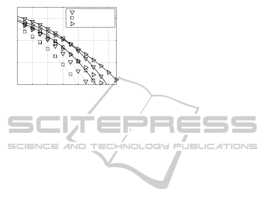
The optimization results when using PA are shown

in Fig. 11 and Fig. 12: The BER becomes minimal

in case of an optimized bit loading with highest bit

loading in the layer with largest singular values.

Fig. 13 and 14 show the MIMO system perfor-

mance when using ﬁxed transmission modes and hav-

ing different degrees of correlation. As highlighted by

the BER curves, in case of high correlation only the

layers with the largest singular values should be used

for the data transmission.

WINSYS2013-InternationalConferenceonWirelessInformationNetworksandSystems

230

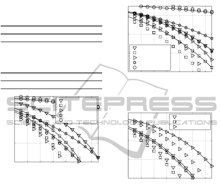
Table 4: Probability of choosing speciﬁc transmission

modes in weakly correlated MIMO channels at a ﬁxed data

rate by using optimal bitloading (10 · log

) = 10

dB).

mode (64,4,0,0) (16,16,0, 0) (16,4, 4,0) (4, 4,4,4)

pdf 0.1274 0.3360 0.5366 0.0

Table 5: Probability of choosing speciﬁc transmission

modes in strongly correlated MIMO channels at a ﬁxed data

rate by using optimal bitloading (10 · log

) = 10

dB)

mode (64,4,0,0) (16,16,0, 0) (16,4, 4,0) (4, 4,4,4)

pdf 0.8252 0.1087 0.0605 0.0

12 14 16 18 20 22 24

−8

−6

−4

−2

10 ·lg(E

) (indB) →

bit-error rate →

(256,0,0,0) QAM

(64,4,0,0) QAM

(16,16,0,0) QAM

(16,4,4,0) QAM

(4,4,4, 4) QAM

Figure 11: BER with optimal PA (dotted line) and without

PA (solid line) when using the transmission modes intro-

duced in Tab. 2 and transmitting 8 bit/s/Hz over frequency

non-selective (4×4) MIMO channels (d

= 1, φ = 30

◦

and

= 1,0) with weak transmitter-side correlation.

5 CONCLUSIONS

This paper has shown the correlation coefﬁcients

characterization of transmitter-side correlated MIMO

channels as well as their performance on the pres-

ence of correlation. The correlation coefﬁcients de-

pend on paths physical parameters describing the an-

tennas arrangement. Antennas spacing, angle of de-

parture and the scattering angle affect the paths cor-

relation degree and hence the MIMO performance.

The singular-value decomposition (SVD) is a signal

processing technique that having perfect channel state

information at both the transmit and receive sides in-

volves pre- and post-processing at the transmit and

receive sides respectively which converts the MIMO

channel into independent layers characterized by the

layer gain given by the singular values. Antennas cor-

12 14 16 18 20 22 24

−8

−6

−4

−2

10 ·lg(E

) (indB) →

bit-error rate →

(256,0,0,0) QAM

(64,4,0,0) QAM

(16,16,0,0) QAM

(16,4,4,0) QAM

(4,4,4, 4) QAM

Figure 12: BER with optimal PA (dotted line) and without

PA (solid line) when using the transmission modes intro-

duced in Tab. 2 and transmitting 8 bit/s/Hz over frequency

non-selective (4×4) MIMO channels (d

= 1/4, φ = 30

◦

and σ

= 1,0) with strong transmitter-side correlation.

12 14 16 18 20 22 24

−8

−6

−4

−2

10 ·lg(E

) (indB) →

bit-error rate →

no Correlation

weak Correlation

strong Correlation

Figure 13: BER with optimal PA (dotted line) and without

PA (solid line) when using the (16,16,0,0 QAM transmis-

sion mode and transmitting 8 bit/s/Hz over frequency non-

selective (4×4) MIMO channels with different degrees of

correlation.

relation affects the SVD dealing to dispersed singular

values: some with large values and others with low

values, in contrast to the ideal case. This singular val-

ues dispersion yields a poor MIMO channel perfor-

mance due to those layers with low singular values

which present a low reliability. The overall anten-

nas correlation effect is described by the correlation

matrix which relates the channel uncorrelated matrix

to the correlated one. The analysis has demonstrated

that the representation of the PDF of the ratio be-

tween the smallest and the largest singular values pro-

vides a useful mean to predict the channel behavior

and the appropriateness of activating all the MIMO

layers. Besides, the singular values CCDF gives rel-

evant information concerning the probability of ob-

Modulation-modeandPowerAssignmentinSVD-assistedMIMOSystemswithTransmitter-sideAntennasCorrelation

231

12 14 16 18 20 22 24

−8

−6

−4

−2

10 ·lg(E

) (indB) →

bit-error rate →

no Correlation

weak Correlation

strong Correlation

Figure 14: BER with optimal PA (dotted line) and without

PA (solid line) when using the (64,4,0, 0 QAM transmis-

sion mode and transmitting 8 bit/s/Hz over frequency non-

selective (4×4) MIMO channels with different degrees of

correlation.

taining predominant (strong and weak) layers and in-

fer the MIMO channel behaviour. The best perfor-

mance is obtained when all CCDF coincide (are the

same) or are quite close. CCDF curve dispersion re-

veals the existence of predominant layer lowering the

MIMO performance. Additionally, in order to miti-

gate correlation effects the investigation has analyzed

the effect of bit and transmit power allocation along

the various MIMO layers as techniques for improv-

ing channel performance even in the presence of an-

tennas correlation. Regarding the power allocation,

a basic technique has been applied in order to obtain

the same quality along the different activated layers,

i.e., the same SNR at each detector. This technique

allows obtaining a higher performance. Moreover, bit

loading has been studied through the description of

some proﬁles (transmission modes) dealing to differ-

ent constellation per layer (bit per symbol interval)

but maintaining the overall transmission rate. A re-

markable conclusion is that activating all the MIMO

layers not necessarily provides the best performance

as highlighted in the results where the transmission

modes (64,4,0, 0) and (16,16, 0,0) present the best

performance. In order to highlight the importance of

this fact the probability of using each transmission

mode was analyzed and the previous conclusion was

remarked.

REFERENCES

Ahrens, A. and Lange, C. (2008). Modulation-Mode and

Power Assignment in SVD-equalized MIMO Sys-

tems. Facta Universitatis (Series Electronics and En-

ergetics), 21(2):167–181.

Cano-Broncano, F., Benavente-Peces, C., Ahrens, A.,

Ortega-Gonzalez, F. J., and Pardo-Martin, J. M.

(2013). Analysis of MIMO Systems with Transmitter-

Side Antennas Correlation. In International Con-

ference on Pervasive and Embedded Computing

and Communication Systems (PECCS), Barcelona

(Spain).

Haykin, S. S. (2002). Adaptive Filter Theory. Prentice Hall,

New Jersey.

Kalet, I. (1987). Optimization of Linearly Equalized

QAM. IEEE Transactions on Communications,

35(11):1234–1236.

K¨uhn, V. (2006). Wireless Communications over MIMO

Channels – Applications to CDMA and Multiple An-

tenna Systems. Wiley, Chichester.

Lee, W.-Y. (1973). Effects on Correlation between two Mo-

bile Radio Base-Station Antennas. IEEE Transactions

on Vehicular Technology, 22(4):130–140.

Mutti, C. and Dahlhaus, P. (2004). Adaptive Power Load-

ing for Multiple-Input Multiple-Output OFDM Sys-

tems with Perfect Channel State Information. In Joint

COST 273/284 Workshop on Antennas and Related

System Aspects in Wireless Communications, pages

93–98, Gothenburg.

Oestges, C. (2006). Validity of the Kronocker Model for

MIMO Correlated Channels. In Vehicular Technology

Conference, volume 6, pages 2818–2822, Melbourne.

Proakis, J. G. (2000). Digital Communications. McGraw-

Hill, Boston.

Salz, J. and Winters, J. H. (1994). Effect of Fading Correla-

tion on adaptive Arrays in digital Mobile Radio. IEEE

Transactions on Vehicular Technology, 43(4):1049–

1057.

Shiu, D., Foschini, G., Gans, M., and Kahn, J. (2000). Fad-

ing Correlation and its Effect on the Capacity of Mul-

tielement Antenna Systems. IEEE Transactions on

Communications, 48(3):502–513.

Wong, C. Y., Cheng, R. S., Letaief, K. B., and Murch, R. D.

(1999). Multiuser OFDM with Adaptive Subcarrier,

Bit, and Power Allocation. IEEE Journal on Selected

Areas in Communications, 17(10):1747–1758.

Zhou, Z., Vucetic, B., Dohler, M., and Li, Y. (2005). MIMO

Systems with Adaptive Modulation. IEEE Transac-

tions on Vehicular Technology, 54(5):1073–1096.

WINSYS2013-InternationalConferenceonWirelessInformationNetworksandSystems

232