Protein Secondary Structure Prediction using an Optimised Bayesian

Classification Neural Network

Son T. Nguyen and Colin G. Johnson

School of Computing, University of Kent, Canterbury, Kent, U.K.

Keywords: Protein Secondary Structure Prediction, Classification Bayesian Neural Network, Optimised Network

Architecture.

Abstract: The prediction of protein secondary structure is a topic that has been tackled by many researchers in the

field of bioinformatics. In previous work, this problem has been solved by various methods including the

use of traditional classification neural networks with the standard error back-propagation training algorithm.

Since the traditional neural network may have a poor generalisation, the Bayesian technique has been used

to improve the generalisation and the robustness of these networks. This paper describes the use of

optimised classification Bayesian neural networks for the prediction of protein secondary structure. The

well-known RS126 dataset was used for network training and testing. The experimental results show that

the optimised classification Bayesian neural network can reach an accuracy greater than 75%.

1 INTRODUCTION

The accurate prediction of protein secondary

structure is an important step to understand protein

folding. A large number of papers have tackled this

problem, with the most common approach being the

use of various machine learning methods to learn the

connection between amino acid sequences and

secondary structure. Some of these approaches use

the amino acid states directly as the input data to

learning, whereas other methods have used the

biophysical features of amino acids, sequence

homology, pattern matching and statistical analyses

of proteins of known structures (Rost and Sander,

1993a), (Rost and Sander, 1993b).

The standard way of presenting this task as a

machine learning problem is as a classification

problem, where each data instance consists of a

number of predictor features (e.g. the neighbouring

amino acid values) and a class drawn from the set

{helix, strand, coil}. The aim of the learned model is

to be able to predict this class for examples not seen

during training.

According to (Holley and Karpus, 1989), the

maximum accuracy of predicting three states

(helices, strands and coils) has a limit, due to the

amount of data available and/or that the secondary

structure is determined by tertiary interactions not

included in the local sequence. Nonetheless, models

have been learned that can predict the class with

reasonable accuracy (65% for simple methods, rising

to around 92% for more sophisticated methods that

use additional data about similar proteins) (Lee et

al., 2012)

This paper describes the use of classification

Bayesian neural networks for the prediction of

protein secondary structure. In the past,

classification Bayesian neural networks have been

proven to be useful for several classification tasks

(Nguyen et al., 2004), (Nguyen et al., 2006), (Penny

and Roberts, 1999) and (Thodberg, 1996). Unlike

the traditional neural network training, the Bayesian

neural network training does not require a validation

set separated from the training subset. As a result, all

of the available data set can be divided into only two

subsets: the training subset and the test subset

(Mackay, 1992a), (Mackay, 1992b). The Bayesian

neural network training also encourages

generalisation as the values of the weight decay

parameters, sometimes known hyper-parameters,

can be well adjusted during the network training

phase. Moreover, Bayesian neural networks allow

users to rank and compare different networks with

different architectures. Therefore, the optimal

network architecture can be easily found based on

evaluating the log evidence of candidate networks

with the Bayesian framework (Penny and Roberts,

1999), (Mackay, 1992b).

451

T. Nguyen S. and G. Johnson C..

Protein Secondary Structure Prediction using an Optimised Bayesian Classiﬁcation Neural Network.

DOI: 10.5220/0004538604510457

In Proceedings of the 5th International Joint Conference on Computational Intelligence (NCTA-2013), pages 451-457

ISBN: 978-989-8565-77-8

 2013 SCITEPRESS (Science and Technology Publications, Lda.)

The structure of the paper is organised as

follows. Section II provides an overview of protein

secondary structure prediction and classification

neural networks. In Section III, the formulation of

classification Bayesian neural networks is briefly

described. In Section IV, the paper gives the

assessment methods for the obtained results. Section

V presents how to train and optimise classification

Bayesian neural networks for predicting three states:

helices, strands and coils. Finally, Section VI

provides a conclusion.

2 PROTEIN SECONDARY

STRUCTURE PREDICTION

AND CLASSIFICATION

NEURAL NETWORKS

Protein structure prediction is the foundation of

protein structure biology. Proteins are

macromolecules made of chains of 20 different

amino acids, which fold into a particular three-

dimensional structure that is distinctive to that

protein. This three-dimensional structure is what

determines the function of a protein. The ultimate

goal is to understand the function of proteins, and

therefore an important step towards this

understanding is to understand the protein structure

and how this relates to its sequence. Biochemists

distinguish four distinct aspects of a protein’s

structure: Primary structure, Secondary structure,

Tertiary structure and Quaternary structure. Protein

Secondary Structure Prediction (PSSP) means

predicting which parts of a protein will form the

large-scale structures known as α-helix, β-strand and

coils, based on the amino acid sequence of a protein

(Mottalib et al., 2010).

In the last two decades, a huge number of

approaches have been taken to the PSSP. In these

works, the probabilistic approaches were the first to

be used. The first attempt at using neural networks

for PSSP was done by Qian and Sejnowski in 1988,

and they obtained an accuracy of 64.3% (Qian and

Sejnowski, 1988). More recent neural network based

approaches have achieved accuracies greater than

70% (Rost and Sander, 1993a), (Jones, 1999). The

most important improvement in these approaches is

to modify the input set to the neural network by

finding similar proteins from a large database, and

forming an input based on the proportion of amino

acid values at each position in the sequence. The aim

of this is to provide more information to the network

about the kind of protein, and to eliminate the

influence of an uncharacteristic amino acid at a

particular position.

This part of the paper will describe how

classification neural networks are used for PSSP.

The primary sequences are used as the network

input. In order to read the input, a moving window

through the sequences needs to be created.

According to (Qian and Sejnowski, 1988), the size

of the moving window should be chosen to be 13 as

this window size has given the best performances

when testing the trained network on the test subset—

this window size has also been found in many

subsequent papers.

In this work, the define secondary structure of

proteins (DSSP) method is used. According to this

method, the secondary structure of each residue

classifies into 8 classes, namely H (α-helix), G (310-

helix), I (π-helix), B (isolated β-bridge), E (extended

β-strand), T (hydrogen bonded turn), S (bend), and

C (not HBEGIT or S). The prediction methods are

assessed for only 3 standard classes associated with

α helices (H), β-strands (E) and coils (C). Hence, 8

classes are reduced to 3. In the literature, there are

four main mappings to perform the reduction

process (Sepideh et al., 2008). These are:

1. H,G  H

E  E

S,T,B,I,C  C

2. H  H

E  E

G,S,T,B,I,C  C

H,G,I  H

E,B  E

S,T,C  C

4. H,G  H

E,B  E

S,T,I,C  C

Here, the method 2 is adopted in this research as

it is considered as the strictest criterion. In order to

encode the secondary structure classes for the

classification, three output units are assigned in our

neural network as binary values as follows

H=[1,0,0], E=[0,1,0], and C=[0,0,1]

The prediction of protein secondary structure

based on a multiple alignment profile of protein

instead of a single sequence has been adopted as a

way to improve the prediction accuracy in several

papers (Rost and Sander, 1993a), (Rost and Sander,

1993b). The aim of this is to improve predictive

power by finding proteins that are similar to the

protein being examined, and modifying the input to

be a mixture of the original protein information and

IJCCI2013-InternationalJointConferenceonComputationalIntelligence

452

(a)

(b)

Figure 1: The PSSM matrix: (a) the raw matrix values, (b)

the matrix values normalised with the standard logistic

function.

that of these similar proteins.

There are two kinds of multiple alignment

profiles: 1) the multiple sequence alignment profiles

(MSAP), 2) the position-specific score matrices

(PSSM) (Sepideh et al., 2008). In this research, the

PSSMs for the RS126 dataset are used and they can

be easily obtained from (Jpred 3), which is a simple

and accurate protein secondary structure prediction

method incorporating two feed-forward neural

networks. The profile matrix has 20xL elements,

where L is the length of the target sequence as

shown in Figure.1. As the values of the feed-

forward neural network inputs can only accept 0 to

1, the raw PSSM needs to be normalised using the

logistic function as shown in equation (1).









(1)

where

is the raw matrix value.

As the window size is 13 with 20 amino acids,

there are 13x20 + 1 = 261 neural network inputs (the

last input for the bias term). There are three output

units corresponding to three states (helix, strand and

other structures (sometimes known as loops or

coils)). The network has a single hidden layer, as

one hidden layer is sufficient to solve every problem

including regression and classification (Bishop,

1995). The optimal number of hidden nodes is

theoretically determined based on the Bayesian

inference discussed in details in Section III.

3 CLASSIFICATION BAYESIAN

NEURAL NETWORKS

Bayesian learning of multi-layer perceptron neural

networks is performed by considering Gaussian

probability distributions of the weights which give

the best generalization (Mackay, 1992a), (Mackay,

1992b). In particular, the weights

in network

are adjusted to their most probable values given the

training data

. Specifically, the posterior

distribution of the weights can be computed using

Bayes’ rule as follows





 



XDp

XwpXwDp

XDwp

|,|

,| 

(2)

where





XwDp ,| is the likelihood function, which

contains information about the weights from

observations, and the prior distribution





Xwp |

contains information about the weights from

background knowledge. The denominator,



XDp | ,

is known as the evidence for network X given data-

set D.

Given a set of candidate networks

X having

different numbers of hidden nodes, the posterior

probability of each network can be expressed as





 



XpXDp

DXp

| 

(3)

If the networks are assumed to be equally probable

before any data is observed, then



Xp is the same

for all networks. Since





Dp does not depend on the

network, then the probable network is the one with

the highest evidence





XDp | . Therefore, the

evidence can be used to compare and rank different

candidate networks.

The weights and biases of the Bayesian neural

network are grouped into a single vector and

determined as follows

1mmmm

ww d









(4)

where



is the weight vector at the training

iteration



is the weight vector at the

training iteration



is the adaptive learning rate

at the training iteration

and

is the search

direction at the training iteration

. The adaptive

learning rate is adjusted during the training phase

based on the Scaled Conjugate Gradient method

(Moller, 1993). In this research, the search direction

ProteinSecondaryStructurePredictionusinganOptimisedBayesianClassificationNeuralNetwork

453

is predefined to be the negative gradient



Regularisation is used to prevent any weights

becoming excessively large, which can lead to poor

generalisation. For a multi-layer perceptron neural

network classifier with

groups of weights and

biases, a weight decay penalty term proportional to

the sum of squares of the weights and biases is

added to the data error function

E to obtain the

cost function

EES









(5)



),...,1( Gg 

(6)

where

is called the cost function,



is a non-

negative scalar, sometimes known as a

hyperparameter, ensuring the distribution of weights

and biases in group

and

is the vector of

weights and biases in group

In network training, the hyperparameters are

initialised to be arbitrary small values. The cost

function is then minimised using the Scaled

Conjugate Gradient method. When the cost function

has reached a local minimum, the hyperparameter



( Gg ,...,1 ) is re-estimated. This task requires

computing the Hessian matrix of the cost function:

IHA









(7)

where

is the Hessian matrix of

E and

the identity matrix, which selects weights in the

group. The number of ‘well-determined’ weights



in group

is calculated based on the old value of



as follows:





ggg g

WtrAI







),...,1( Gg 

(8)

The new value of the hyperparameter



is then re-

estimated as







),...,1( Gg 

(9)

The hyperparameters need to be re-estimated several

times until the cost function value ceases to change

significantly between consecutive re-estimation

periods. After the network training is completed, the

values of parameters



and



are then used to

compute the log evidence of network

X having

hidden nodes as follows (Penny and Robert, 1999):

























lnln

2ln!lnln

MMA

SXEv







(10)

where

is the number of weights and biases in

group

, and



is set to be

10 (Thodberg, 1996).

However,



is a minor factor because it is the same

for all models and therefore does not effect to the

relative comparison of log evidence of different

network architectures. Equation (10) is used to

compare different networks having different

numbers of hidden nodes. The best network will be

selected with the highest log evidence.

4 EVALUATION METHODS

A useful accuracy evaluation for classification

neural networks is well-known three state overall

residue accuracy percentage defined as follows

100

loop

PPP







(11)

where





and

loop

are the number of correctly

predicted



-helix,



-sheet and loop, respectively.

is the total number of residues in a given protein

sequence.

Another widely used accuracy measurement is

the Matthew’s correlation coefficients. In the case of



helix, this coefficient is determined as follows



pn uo

nuno pu po

 









 

(12)

where



is the number of correctly predicted

positive cases,



is the number of correctly

rejected negative cases,



is the number of over-

predicted cases (false positives), and



is the

number of under-predicted cases (misses). Similarly,



and

loop

can be also defined for



-sheet and

loop, respectively. If the coefficients are equal to 1,

the model predictions are 100% correct. Whereas, if

the coefficients are equal to -1, the model

predictions are 100% incorrect.

IJCCI2013-InternationalJointConferenceonComputationalIntelligence

454

5 EXPERIMENTS AND RESULTS

The RS126 dataset was used for training and testing

the networks (Rost and Sander, 1993a). All of the

dataset was randomly divided into seven subsets. A

seven fold cross-validation technique was applied to

determine the prediction accuracy. In particular, six

subsets were used for training networks and the

remaining subset was used for testing networks. This

procedure was repeated for the different test subsets.

Bayesian neural networks with different numbers of

hidden nodes were trained to select the optimal

network architecture. These networks have the

following specification, as discussed in detail earlier

in the paper:

 four hyperparameters



and



constrain the magnitudes of the weights on the

connection from the input nodes to the hidden

nodes, the biases of the hidden nodes, the weights

on the connection from the hidden nodes to the

output nodes, and the biases of the output nodes;

 261 inputs, corresponding to 20 inputs for each

letter in the moving with the size is 13 and one

bias term with a constant value of 1;

 three outputs, each corresponding to one of the

states: helix, strand and other structures.

For a given number of hidden nodes, five

networks with different initial values of the weights

and biases were trained. The training procedure was

implemented as follows:

1. The weights and biases in four different groups

were initialised by random selections from zero-

mean, unit variance Gaussians and the initial

hyperparameters were chosen to be small values.

2. The network was trained to minimise the cost

function

using Scaled Conjugate Gradient

training algorithm.

3. When the network training had reached a local

minimum, the values of the hyperparameters

were re-estimated according to equation (8) and

(9).

4. Steps 2 and 3 were repeated until the cost

function value was smaller than a pre-determined

value and did not change significantly in

subsequent re-estimations.

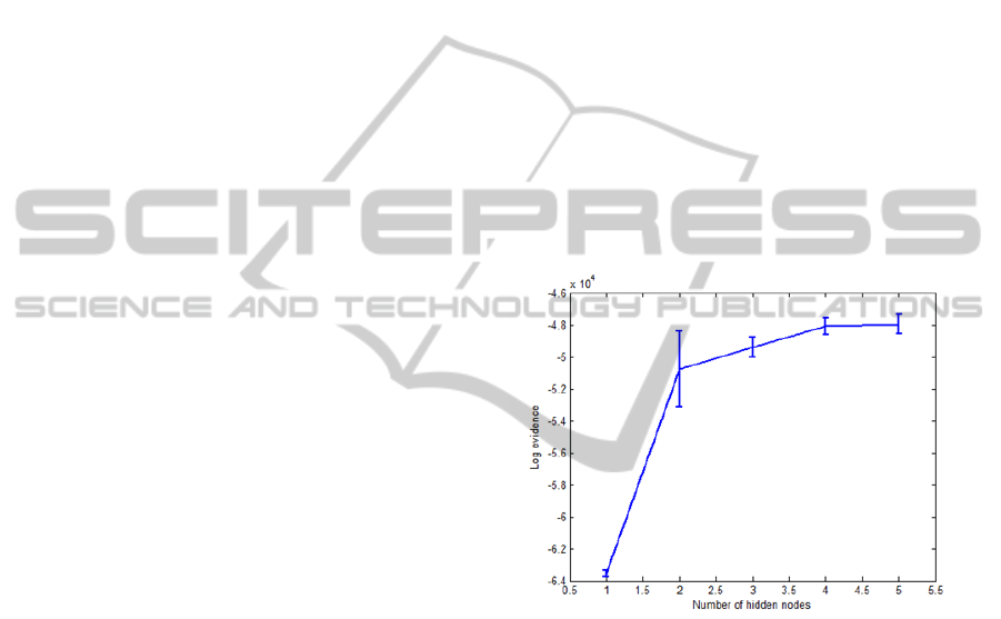
The performances of the trained networks were

tested on the seventh subset. As shown in Figure 2,

the networks having four hidden nodes is the last

increase that produces a meaningful increase in log

evidence. This means that four hidden nodes are

sufficient to solve the problem. Table 1 shows the

change of hyperparameters according to the periods

of re-estimation of a specific network training run.

For each period, there are 100 predefined

trainingiterations.

Table 2 shows the prediction accuracy and the

Matthew’s correlation coefficients on three states

from the classification Bayesian neural network. We

can see that the accuracy is 75.77%. Next, a standard

classification neural network that has the same

structure with the classification Bayesian neural

network was trained to obtain the three-state

prediction accuracy. However, the prediction

accuracy of the trained classification standard neural

network 74.97% and the Matthew’s correlation

coefficients, shown in Table 3, are also smaller than

those of the trained classification Bayesian neural

network shown in Table 2. Whilst this increase is

small, progress in this area has typically come from

the accumulation of small improvements, which can

be combined together to make a larger improvement.

Figure 2: Log evidence versus number of hidden nodes:

The solid curve shows the evidence averaged over the five

networks.

6 CONCLUSIONS

The results obtained show that Bayesian neural

networks can be used to predict the protein

secondary structure with the maximum accuracy of

75.77%. This is better than the traditional neural

network training methods. According to the obtained

results, the use of four hidden nodes is an optimal

choice for the network architecture. This number of

hidden nodes can give the best generalisation of the

trained network without the use of a validation set.

Therefore, the available data was only divided into

two subsets: one for training and another for testing.

Moreover, Bayesian training for neural network can

ProteinSecondaryStructurePredictionusinganOptimisedBayesianClassificationNeuralNetwork

455

automatically adjust the hyperparameters during the

training phase.

The procedure for determining the optimal

structure of the classification standard neural

network (the growing and pruning technique) has

not been mentioned in this paper as this approach

requires a lot of statistical tasks. The main

disadvantage of the Bayesian learning for feed-

forward neural networks is that it takes a quite long

time on evaluating the Hessian matrix, especially

when the number of network parameters (weights

and biases) is relatively large.

Table 1: The change of hyperparameters according to the

periods of re-estimation.

Periods



1 31.392 1.371 0.529 0.775

2 99.919 2.389 0.334 2.432

3 198.498 4.055 0.231 3.949

Table 2: The three-state prediction accuracy and

Matthew’s correlation coefficients of classification

Bayesian neural network.

Matthew’s Correlation

Coefficients

Fold

(%)Q C





loo

A 75.840 0.699 0.531 0.565

B 78.187 0.728 0.607 0.604

C 72.422 0.635 0.510 0.524

D 75.319 0.658 0.550 0.540

E 74.826 0.641 0.580 0.542

F 76.362 0.697 0.598 0.569

G 77.462 0.696 0.578 0.604

Average 75.774 0.679 0.565 0.564

Table 3: The three-state prediction accuracy and

Matthew’s correlation coefficients of standard

classification Bayesian neural network.

Matthew’s Correlation

Coefficients

Fold

(%)Q C





loo

A 75.927 0.689 0.543 0.565

B 77.347 0.725 0.583 0.587

C 71.321 0.619 0.496 0.502

D 74.826 0.646 0.551 0.536

E 73.812 0.622 0.571 0.521

F 74.739 0.669 0.572 0.548

G 76.796 0.669 0.568 0.604

Average 74.967 0.663 0.555 0.552

REFERENCES

B. Rost and C. Sander, "Prediction of protein secondary

structure at better than 70% accuracy," J.Mol.Biol.,vol.

232, pp. 584-599, 1993a.

B. Rost and C. Sander, "Improved prediction of protein

secondary structure by use of sequence profiles and

neural networks.," Proc, Natl, Acad, Sci, Biophysics,

USA, pp. 7558 - 7562, 1993b.

L. H. Holley and M. Karpus, "Protein secondary structure

prediction with a neural network," Proc, Natl, Acad,

Sci, Biophysics, USA, vol. 86, pp. 152 - 156, 1989.

L. Lee, J. L. Leopold, and R. L. Frank, "Protein secondary

structure prediction using BLAST and exhaustive RT-

RICO, the search for optimal segment length and

threshold," 2012 IEEE Symposium on Computational

Intelligence in Bioinformatics and Computational

Biology (CIBCB), pp. 35 – 42, 2012.

S. T. Nguyen, H. T. Nguyen, and P. Taylor, "Hands-Free

Control of Power Wheelchairs using Bayesian Neural

Networks," Proceedings of IEEE Conference on

Cybernetics and Intelligent Systems, Singapore, 2004,

pp. 745 - 749, 2004.

S. T. Nguyen, H.T.Nguyen, P. Taylor, and J. Middleton,

"Improved Head Direction Command Classification

using an Optimised Bayesian Neural Network,"

Proceedings of IEEE International Conference of the

Engineering in Medicine and Biology Society, New

York City, New York, USA, August 30-Sept. 3, 2006.

W.D. Penny and S. J. Roberts, "Bayesian neural networks

for classification: how useful is the evidence

framework," Neural Networks, vol. 12, pp. 877 - 892,

1999.

H. H. Thodberg, "A review of Bayesian neural networks

with an application to near infrared spectroscopy,"

IEEE Transactions on Neural Networks, vol. 7, pp. 56

- 72, 1996.

D. MacKay, "A practical Bayesian Framework for

Backpropagation Networks," Computation and Neural

Systems, vol. 4, pp. 448-472, 1992a.

D. MacKay, "The Evidence Framework Applied to

Classification Networks," Neural Computation, vol. 4,

pp. 720 -736, 1992b.

C. M. Bishop, "Neural networks for pattern recognition,"

Oxford: Clarendon Press; New York: Oxford

University Press, 1995.

M. A. Mottalib, M. S. R. Mahdi, A. B. M. Z. Haque, S. M.

A. Mamun, and H. A. Al-Mamun, "Protein Secondary

Structure Prediction using Feed-Forward Neural

Network," JCIT, vol. 1, pp. 64 - 68, 2010.

N. Qian and T. J. Sejnowski, "Predicting the Secondary

Structure of Globular Proteins Using Neural Network

Models," J. Mol. Biol. 202, pp. 865 - 884, 1988.

M. F. Moller, "A Scaled Conjugate Gradient Algorithm

for Fast Supervised Learning," Neural Networks, vol.

6, pp. 525 - 533, 1993.

Jpred 3, http://www.compbio.dundee.ac.uk/www-jpred/

David T. Jones, "Protein Secondary Structure Prediction

Based on Position-specific Scoring Matrices,"

J.Mol.Biol.,vol.292, pp.195-202, 1999.

IJCCI2013-InternationalJointConferenceonComputationalIntelligence

456

B. Sepideh, S. S. Ali, and G. A. R, "Pruning neural

networks for protein secondary structure prediction,"

8th IEEE International Conference on BioInformatics

and BioEngineering, 2008. BIBE 2008, pp. 1 - 6,

2008.

K. Rajasekhar, D. V. Kumar, and O. O. Ahmad, " A two-

stage neural network based technique for protein

secondary structure prediction " The 2nd International

Conference on Bioinformatics and Biomedical

Engineering, 2008. ICBBE 2008, pp. 1355 - 1358

2008.

ProteinSecondaryStructurePredictionusinganOptimisedBayesianClassificationNeuralNetwork

457