
Trajectory Pattern Mining in Practice
Algorithms for Mining Flock Patterns from Trajectories
Xiaoliang Geng
1
, Takeaki Uno
2
and Hiroki Arimura
1
1
Graduate School of IST, Hokkaido University, N14 W9, Kita-ku, Sapporo 060-0814, Japan
2
National Institute of Informatics, Hitotsubashi, Chiyoda-ku, Tokyo 101-8430, Japan
Keywords:
Trajectory Mining, Spatio-temporal Mining, Depth-first Mining Algorithm, Frequent Itemset Mining.
Abstract:
A flock pattern is a spatio-temporal pattern that represents a group of moving objects which are close to each
other in a given time segment (Gudmundsson and van Kreveld, Proc. ACM GIS’06; Benkert, Gudmundsson,
Hubner, Wolle, Computational Geometry, 41:11, 2008). In this paper, we give empirical study of our recent
development of a flock pattern mining algorithm FPM and its modifcations, which are the first purely depth-
first algorithms for flock pattern mining. We implemented two extensions of the basic FPM algorithm, one is
RFPM for a class of closed patterns, called rightward length-maximal flock patterns, and the other is G-RFPM
with a speed-up technique using geometric indexes. To evaluate their performance, we ran experiments on
synthetic datasets. The experiments demonstrate that the modified algorithms with the above extensions are
several order of magnitude faster than the original algorithm in most parameter settings.
1 INTRODUCTION
1.1 Background
By the rapid progress of mobile devicesand positional
sensors, a massive amount of trajectory data, which
are collections of sequences of real-valued locations
with errors and missing values, have been accumu-
lated. Since mining of trajectory data have different
characteristics from traditional transaction data min-
ing (Pei et al., 2004), research of trajectory mining has
attracted a great deal of attention for recent years (Gi-
annotti et al., 2007; Vieira et al., 2009).
A trajectory database on a time domain T = [1, T]
is a collection S of n trajectories for n moving objects,
such as wild animals, walking people, or floating cars,
where each trajectory is a sequence of T points on the
2-dimensional space R
2
to which an index called a
trajectory ID is associated. A flock pattern is a spatio-
temporal pattern, introduced by (Gudmundsson and
van Kreveld, 2006), defined as follows. For r > 0
and k, m ≥ 0, called min-len and min-sup, an (r, k, m)-
flock pattern in S is a pair P = (X,[b,e]) of a set X
of trajectory ids and a time interval I = [b,e] in T that
represents a set of at least m movingobjects that move
together in a continuous interval of length at least k
time points in mutual distance at most r in L
∞
-norm
1
.
Most of previous studies on mining flock pat-
terns (Benkert et al., 2008; Gudmundsson and van
Kreveld, 2006; Laube et al., 2005) deal with only
searching flock patterns in a given trajectory data,
but not mining them. For mining the complete set
of flock patterns with given constraints, (Vieira et al.,
2009) presented a micro-cluster based mining algo-
rithm with memorization, and (Romero, 2011) stud-
ied a mining algorithm built on the top of an existing
frequent itemset mining algorithm LCM (Uno et al.,
2004). Although their algorithms seem depth-first
search algorithms, they do not work in purely depth-
first manner since they require to store intermediate
results on main memory.
In this paper, we focus on pattern-growth ap-
proach for the problem of finding all (r, k)-flock pat-
terns. We develop the first purely depth-first algo-
rithm FPM that can make the complete mining of
flock patterns (Arimura et al., 2013). Particularly, this
paper presents two extensions RFPM and G-RFPM of
of FPM. The first one, RFPM, finds a class of closed
patterns, called rightward length-maximal flock pat-
terns, while the second one, G-RFPM, uses speed-up
1
Our (r, k,m)-flock patterns use L
∞
-distance on R
2
,
while the original (m,k, r)-flock patterns of Benkert et
al. (Benkert et al., 2008) used L
2
-distance on R
2
143
Geng X., Uno T. and Arimura H..
Trajectory Pattern Mining in Practice - Algorithms for Mining Flock Patterns from Trajectories.
DOI: 10.5220/0004543401430151
In Proceedings of the International Conference on Knowledge Discovery and Information Retrieval and the International Conference on Knowledge
Management and Information Sharing (KDIR-2013), pages 143-151
ISBN: 978-989-8565-75-4
Copyright
c
2013 SCITEPRESS (Science and Technology Publications, Lda.)

Figure 1: Examples of a trajectory database S
1
on ID =
{1,. . . ,5} and T = [1, 7] and a (1.0, 2, 2)-flock pattern P
1
=
(X
1
,I
1
) = ({2, 3,4},[3, 5]) with diameter ||P
1
||
∞
S
1
≤ 1.0,
length len(P
1
) = 3, and support supp(P
1
) = 3. Here, each
line indicates a trajectory and the numbers attached to points
are time stamps.
technique using geometric indices.
We implemented the basic and the improved al-
gorithms above based on pattern-growth mining ap-
proach. To evaluate these extensions, we then ran ex-
periments on implanted synthetic datasets. The ex-
periments demonstrated that both of extensions sig-
nificantly improve on the efficiency of the original al-
gorithm FPM in a wide range of parameter settings.
For example, in the case of a trajectory database
with 200K points, where C = 5 copies of K = 6 hid-
den patterns are embedded into 200 trajectories of
length 1K points, the running times for FPM, RFPM,
and G-RFPM found all patterns in 61.61, 0.96, and
0.03 seconds, respectively. From these results, we ob-
tained around 60 and 30 times speed-ups by the first
and second extensions, respectively, and finally, the
total speed-up becomes around 2,000 times.
This paper is organized as follows. Sec.2 gives
definitions for flock pattern mining including our
rightward length-maximal flock patterns. Sec.3
presents the basic algorithm as well as two improve-
ments. Sec.4 is a main section of this paper that shows
experimental results. Finally, Sec.5 concludes.
2 PRELIMINARIES
2.1 Basic Definitions
Let R and N be the set of all real numbers and all non-
negative integers, respectively. For integers a, b (a ≤
b), we denote by [a, b] = {a,a+ 1, . .. , b} the discrete
interval between a and b. If a,b ∈ R, a ≤ b, then [a, b]
denotes a continuous interval in R as usual. For a set
A, |A| denotes the cardinality of A, and A
∗
denotes the
set of all possibly empty, finite sequences over A.
2.2 Trajectory Database
Let n and T ≥ 0 are pre-determined nonnegative in-
tegers, which indicate the number of moving objects
and the maximum value for discrete time stamps, re-
spectively. Let R
2
be the 2-dimensional continuous
space, or the plane.
A trajectory database on the space domain R
2
and the time domain T = {1, .. . ,T} is a finite
set S = { s
i
|i = 1, .. . ,n } ⊆ (R
2
)
T
of the trajecto-
ries for n moving objects o
1
,. . . ,o
n
, where for ev-
ery i = 1, ... ,n, (i) the index i, called the trajec-
tory ID, is drawn from a set of n identifiers ID =
{1, .. . ,n}, and (ii) the i-th trajectory s
i
is a se-
quence s
i
= s
i
[1]·· · s
i
[T] ∈ (R
2
)
T
of T points on the
2-dimensional space R
2
such that its t-th point is
s
i
[t] = (x
it
,y
it
) ∈ R
2
.
2.2.1 Example 1
In Fig. 1, we show an example of a trajectory database
S, which consists of five trajectories of length T = 7.
For example, GPS-trajectories of wild animals,
walking people with Wifi device, Probe car data (or
floating car data) are instances of such trajectory
databases.
2.3 The Class of Flock Patterns
For such trajectory databases, we introduce the class
F P of spatio-temporal patterns, called flock patterns,
based on L
∞
-norm as follows
2
. Formally, the class of
flock patterns is defined as follows.
Definition 1 (FP). A flock pattern on T is a pair P =
(X, [b, e]), where (i) X ⊆ ID is a finite set of ids, called
the ID set of P, and (ii) I = [b, e] is a discrete interval
in [0, T] with b ≤ e ≤ T, where b and e are called the
start and end time of P.
We define the support, length, and width of a flock
pattern as follows. (i) The support of P, denoted by
supp(P), is defined by the number of trajectory (ID)
contained in X, that is, supp(P) = |X|. (ii) The length
of P, denoted by len(P), is the width of the interval
I, that is, len(P) = e − b + 1. Clearly, we have 0 ≤
supp(P) ≤ n and 0 ≤ len(P) ≤ T.
2.3.1 Example 2
In Fig. 1, we show an example of a flock pattern
P
1
= (X
1
,I
1
), where the ID set is X
1
= {2, 3,4} and
the interval is I
1
= [3, 5].
2
The original version of flock patterns are defined based
on L
2
-norm in (Laube et al., 2005; Gudmundsson and van
Kreveld, 2006).
KDIR2013-InternationalConferenceonKnowledgeDiscoveryandInformationRetrieval
144

To define the width, we require some definitions
below. For a point p = (x, y) on 2-dimensional plane
R
2
, the x- and y-coordinates of p are denoted by by
p.x = x and p.y = y, respectively. For two points p
and p
′
on R
2
, we denote the L
∞
-distance between p
and p
′
by L
∞
(p, p
′
) = max{|p.x− p
′
.x|,|p.y− p
′
.y|}.
By definition, L
∞
(p, p
′
) is nonnegative, and coincides
zero if and only if p = p
′
.
The diameter of a set A = {p
1
,. . . , p
n
} of points,
denoted by ||A||
∞
, is the maximum L
∞
-distance be-
tween any two points in A, defined by
||A||
∞
= max
p,p
′
∈A
L
∞
(p, p
′
), (1)
The width || A||
∞
of a set A is always nonnegative,
and equals zero if and only if A consists of a single
point. We can show that || A||
∞
is linear time com-
putable in n = |A| on R
2
. For any d ≥ 2, ||A||
∞
can
be computed O(dn) time in R
d
, which is still linear in
n for fixed d.
In an input database S, the t-th time slice, denoted
by S[X][t], is the set of all points that appear in the
trajectories of X with time stamp t. The width ||P||
S
∞
of a flock pattern P = (X,I) = (X, [b, e]) is defined by
the maximum diameter of the t-th time slice of the
trajectories in X over all t ∈ [b, e]. Actually, we have
the next lemma.
Lemma 1. The width of P can be computed by Al-
gorithm 1 in O(mℓ) time, where m = supp(X) is the
support of P and ℓ = len(P) is the length of P.
Algorithm 1: Computing the width || P||
∞
S
of a flock pat-
tern P = (X, [b,e]) in a database S = { s
i
|i = 1,. .. ,n}.
1: width ← 0;
2: for t ← b,b+ 1, .. ., e do
3: S
t
← { s
i
[t] |i ∈ X }; ⊲ the t-th slice
4: width ← max{width, ||S
t
||
∞
};
5: return width;
Let r > 0 be a positive number, and k, m ≥ 0 are
non-negativeintegers, respectively, called a maximum
width (max-width), a minimum length (min-len), and
a minimum support (min-sup) parameters.
Definition 2. An r-flock pattern is any flock pattern
P such that ||P||
∞
≤ r, An (r, k)-flock pattern is any
r-flock pattern P with len(P) ≥ k.
2.3.2 Example 3
The pattern P
1
of Fig. 1 in the last example has diam-
eter ||P
1
||
∞
S
1
≤ 1.0, length len(P
1
) = 3, and support
supp(P
1
) = 3. Thus, it is a (1.0, 2,3)-flock pattern for
r = 1.0, k = 2, and m = 3.
In this paper, we consider all (r, k)-flock patterns
in a given trajectory database.
2.4 Rightward Length-maximal
Patterns
For a given max-width parameter r ≥ 0, it is often
useful to find only (r,k)-flock patterns P = (X, [b, e])
whose time interval [b, e] are extended rightward
along time line as long as possible preserving the
diameter r (See (Gudmundsson and van Kreveld,
2006)). This idea of length-maximal mining is ex-
pected to reduce the number of solutions and running
time than just finding all (r, k)-patterns.
A flock pattern P = (X, [b, e]) is said to be a right-
ward length-maximal flock pattern in S if its interval
cannot be extended rightward without changing the
width of P in S.
Formally, it is defined as follows.
Definition 3 (RFP). A flock pattern P = (X, [b, e]) in
S is a rightward length-maximal flock pattern (RFP,
for short) if there is no other flock pattern P
′
=
(X, [b, e
′
]) in S such that (i) P
′
has the same ID set
X as P, and (ii) the right end of P
′
is strictly more
larger than that of P.
By definition, any RFP in S is an FP. However, the
converse does not hold in general. Thus, we have the
inclusion R F P (r, k) ⊆ F P (r, k).
2.4.1 Example 4
In the example of Fig. 1, the flock pattern P
1
=
(X
1
,[3,5]) of length three is an RFP in S
1
, while
P
2
= (X
1
,[3,4]) and P
3
= (X
1
,[3]) are non-rightward
length-maximal FPs, where X
1
= {2, 3, 4}. On the
other hand, P
1
has RFPs P
4
= (X
1
,[4,5]) and P
5
=
(X
1
,[5]).
2.5 The Data Mining Problems
For any class name C ∈ {F P ,R F P ,. . .} and any pa-
rameter values r, k ≥ 0, we denote by C(r, k) the class
of all (r,k)-flock patterns within the class C . Sim-
ilarly, we define the classes C (r), and C (r, k, m) as
well. From now on, we consider the classes F P (r,k)
and R F P(r, k).
We state our data mining problem as follows.
Definition 4. (FLOCK PATTERN MINING PROBLEM
FOR PATTERN CLASS C ) Let C be a class of flock
patterns. An input is a tuple (S,r, k) of an input trajec-
tory database S, and parametervalues r and k ≥ 0. The
task is to find all flock patterns P in S within class C
without repetition that have width at most r and length
at least k.
TrajectoryPatternMininginPractice-AlgorithmsforMiningFlockPatternsfromTrajectories
145

Algorithm 2: A basic DFS algorithm FPM for finding all
(r, k)-flock patterns in an input trajectory database S given
maximum width r and minimum length k.
1: procedure FPM(ID, S, r, k)
2: for ℓ ← k, ... ,T do ⊲ Every length
3: for b
0
← 1,.. . ,T do ⊲ Each start time in T
4: ℓ
0
← b
0
+ ℓ − 1;
5: ID
1
← ID;
6: while ID
1
6=
/
0 do ⊲ Each id in ID
7: i
0
= deletemin(ID
1
);
8: P
0
← ({i
0
}, [b
0
,ℓ
0
]); ⊲ Initial pattern
9: RecFPM(P
0
,ID
1
,S, r, k);
10: procedure RECFPM(P = (X, [b, e]),ID,S, r, k)
11: if ||P||
∞
S
> r then
12: return ; ⊲ P is too wide
13: output P;
14: ID
1
← ID;
15: while ID
1
6=
/
0 do
16: i = deletemin(ID
1
);
17: RecFPM(Q = (X ∪ {i},[b,e]), ID
1
,S, r, k);
18: end while
Similarly, we can consider the flock pattern min-
ing problem with parameters (r, k, m).
We evaluate the performance of a flock pattern
mining algorithm A in terms of enumeration algo-
rithms (Avis and Fukuda, 1993). Let N and M be the
input size and the number of patterns as solutions. A
pattern mining algorithm A is said to have polynomial
delay (poly-delay) if the delay, which is the maximum
computation time between two consecutiveoutputs, is
bounded by a polynomial p(N) in N. A is of polyno-
mial space (poly-space) if the maximum size of its
working space, in addition to that of output stream O,
is bounded by a polynomial p(N).
3 ALGORITHMS
In this section, we present our pattern mining algo-
rithms for FPs and RFPs. We also give a speed-up
technique using geometric indexes to prune redundant
candidates.
3.1 A Basic DFS Algorithm for FPs
We first present a basic mining algorithm FPM (ba-
sic flock pattern miner) for FPs. In Algorithm 2
we present the algorithm FPM with its subprocedure
RecFPM for mining (r, k)-FPs.
In the overall design of our algorithm FPM, we
employ DFS (depth-first search) procedure according
to pattern growth approach (e.g., (Pei et al., 2004)) ap-
proach, as in PrefixSpan (Pei et al., 2004), Eclat (Zaki,
2000) and LCM (Uno et al., 2004).
In DFS (or pattern growth) approach, a recursive
mining procedure searches for all descendant of the
current pattern from smaller to larger in depth-first
manner using backtracking. The advantage of DFS
approach is that DFS miners are proven fast in main
memory environment and can be easily implemented
as a simple recursive procedure.
At the top-level of FPM, for each possible length
ℓ ∈ [k,T] no less than k, it invokes the recursive sub-
procedure RecFPM given as arguments an initial pat-
tern P
0
= (X
0
,[b
0
,e
0
]) consisting of a singleton ID set
X
0
= {i
0
} and an interval [b
0
,e
0
] for every possible
combination of i
0
∈ ID and b
0
∈ [0, T]. The end time
e
0
is calculated by b
0
and ℓ.
The recursive subprocedure RecFPM is a DFS al-
gorithm (or a backtracking algorithm) that searches
the hypothesisspace of all r-flock patterns with length
exactly ℓ as follow.
Starting from the initial pattern P
0
= (X
0
,[b
0
,e
0
])
consisting of a singleton ID set X
0
= {i
0
}, the
procedure enumerates all subsets X of ID using a
backtracking algorithm similar to depth-first search
algorithms for frequent itemset mining, such as
Eclat (Zaki, 2000) and LCM (Uno et al., 2004).
For each generated subset X, the procedure forms
a candidate (r, k)-flock pattern P = (X, [b, e]) with a
specified interval [b, e]. Then, the algorithm computes
the width ||P||
∞
of the pattern P by accessing the tra-
jectories in S, and checks if P satisfies the width con-
straint || P||
∞
≤ r. If the condition is violated, then it
prunes the search for P and all of its descendants.
This width-based pruning rule is justified by the
following lemma, which says the class of (r, k)-
patterns has the anti-monotonicity w.r.t. set inclusion
of their ID sets.
Lemma 2 (anti-monotonicity). Let P
i
= (X
i
,I
i
) be two
flock patterns, where i = 1, 2. If P
2
is an (r, k)-flock
pattern in S and if X
1
⊆ X
2
and I
1
⊆ I
2
hold, then P
1
is also an (r, k)-flock pattern in S.
From this lemma, once a candidate pattern P =
(X, I) does not satisfy the width and length con-
straints, any descendant of P obtained by adding new
trajectory (ids) to X no longer satisfies the constraints.
Therefore, we can prune the whole search sub-space
for descendants of P for (r, k)-flock patterns.
On the running time and space of the algorithm
FPM, The following proposition is easily derived
from our manuscript (Arimura et al., 2013).
Proposition 1. (Arimura et al., 2013) Let S be an in-
put trajectory database S of n trajectories with length
T. Then, the algorithm FPM in Algorithm 2 solves the
KDIR2013-InternationalConferenceonKnowledgeDiscoveryandInformationRetrieval
146

flock pattern mining problem for the class F P M (r,k)
of (r,k)-flock patterns in S. It uses O(knT
2
) time per
pattern and O(k
2
) words of space, respectively, where
k = supp(X) = |X| is the support of the pattern X be-
ing enumerated.
From the practical view, O(T
2
) term in the time
complexity of FPM is too large to apply it to long tra-
jectories with large T. We point that this O(T
2
) term
come from the doubly nested for-loop in Lines 2 and 3
of Algorithm 2. In the next subsection, we will see
how we can remove this O(T
2
) term by focusing on
mining of RFPMs.
3.2 A Modified Algorithm for RFPs
Next, we present a modified mining algorithm RFPM
(rightward flock pattern miner) for RFPs (rightward
length-maximal flock patterns), the class of rightward
length-maximal flock patterns. In Algorithm 4, we
present the algorithm RFPM with its subprocedure
RecRFPM for mining (r, k)-RFPs.
3.2.1 Rightward Horizontal Closure
From the view of frequent pattern mining, RFPs in a
trajectory database are a sort of closed patterns, which
have been extensively studied in frequent itemset
mining (FIM) field (Uno et al., 2004; Zaki and Hsiao,
2005) as well as formal concept analysis (FCA) field.
Many efficient closed pattern mining algorithms use
a class of operation, called closure operation, which
enlarge a given, possibly non-closed pattern to obtain
its closed version.
For RFPs, we actually havea rightward horizontal
closure operation that extends the interval of a given
non RFPs to obtain a proper RFP.
Definition 5 (rightward horizontal closure). Let P =
(X, I = [b,e]) be any flock pattern in a database S.
Then, the rightward horizontal closure of P in S, de-
noted by RH Closure(P;S, r), is the unique flock pat-
tern P
max
= (X,I = [b, e
max
]) such that e
max
∈ [0,T] is
the maximum value of end position e
′
satisfying the
equality
||P
′
= (X, [b, e
′
])||
∞
= ||P||
∞
. (2)
Note that the rightward horizontal closure opera-
tion only change the end position e, but not change
the ID set X or starting time b of the original P at all.
In Algorithm 3, we show the procedure
RH
Closure that computes the rightward hori-
zontal closure of non-RFP P in O(kℓ) time, where
k = supp(P) = |X| = O(n) and ℓ = len(P
max
) = O(T).
The following lemmas show the correctness of the
rightward horizontal closure. First, the key of the cor-
Algorithm 3: An algorithm for computing the unique right-
ward length-maximal flock pattern. Note that ||S[X][t]||
∞
is
defined to be ∞ for t 6∈ [1, T].
1: procedure RH CLOSURE((X,[b
0
,e
0
]);S, r)
2: t ← b
0
;
3: while ||S[X][t]||
∞
≤ r do
4: t ← t + 1;
5: b ← b
0
; e ← t − 1;
6: return (X, [b, e]);
rectness is the following characterization, which can
be easily shown from definition of RFPs.
Lemma 3 (characterization). Let P = (X, [b, e]) be an
(r, k)-flock pattern in S. Then, P is rightward length-
maximal if and only if
• || S[X][t]||
∞
≤ r for all t ∈ [b, e], and
• || S[X][e+ 1]||
∞
> r,
where we extend the t-th time slice ||S[X][t]||
∞
to be ∞
if either t < 1 or t > T holds for convenience.
From the above lemma, we have the correctness
below.
Lemma 4. (Arimura et al., 2013) The rightward
horizontal closure P
max
of a possibly non-rightward
length-maximal r-FP P is the unique longest r-RFP
such that the ID sets and the start time are identical
to those of P.
Since len(P
max
) ≥ len(P) always holds for P
max
,
we see that if P satisfies the (r, k)-constraint then
so does the obtained RFP P
max
. Hence, P
max
is the
unique longest (r, k)-RFP version of P that share the
ID set and start time.
3.2.2 Putting them Together
We describe the computation done by the algorithm
RFPM. The overall structure of RFPM is almost iden-
tical to the basic algorithm FPM. Given a database S,
the main algorithm RFPM invokes the recursive sub-
procedure RecFPM with an initial pattern P
0
as be-
fore.
Only the difference in the top level is that RFPM
iterates only O(T) iteration here for the start position
b
0
rather than O(T
2
) iteration in FPM using an ini-
tial pattern P
0
= ({i
0
}, b
0
,∗) with missing end posi-
tion e
0
= ∗, called a partial pattern here.
The computation of the recursive subprocedure
RecRFPM proceeds in the following steps.
• Receiving a partial RFP P
∗
= (X,b,∗) as argu-
ments, the recursive procedure RecFPM computes
the rightward horizontal closure P = (X,[b, e])
from P
∗
by the procedure RH
Closure with max-
width r.
TrajectoryPatternMininginPractice-AlgorithmsforMiningFlockPatternsfromTrajectories
147

Algorithm 4: An algorithm RFPM for finding all length-
maximal (r, k)-flock patterns appearing in a given trajectory
database S with ID for maximum width r and minimum
length k.
1: procedure RFPM(ID,S, r, k)
2: for b
0
← 1,.. . ,T do ⊲ Each start time in T
3: for i
0
← 1, ... ,n do ⊲ Each id in ID
4: P
0
= ({i
0
}, [b
0
,∗]);
5: RecRFPM(P
0
,ID,S, r, k);
6: procedure RECRFPM(P = (X,[b, ∗]), ID,S, r, k)
7: P = (X, [b, e]) ← RH Closure((X,[b,∗]);S, r);
8: if len(P) < k then
9: return ; ⊲ P is not an (r, k)-flock pattern
10: output P;
11: ID
1
← ID;
12: while ID
1
6=
/
0 do
13: i = deletemin(ID
1
);
14: P
1
= (X ∪{i}, [b, ∗]);
15: RecRFPM(P
1
,ID
1
,S, r, k);
16: end while
• Next, if the obtained RFP P satisfies (r,k)-
constraints, then output it. Otherwise, we safely
prune all descendants as before.
• Finally, RecFPM recursivelycalls its copy with an
extended pattern P
1
= (X ∪ {i}, [b, ∗]). To avoid
duplicated generation of patterns, the id i is re-
moved from the universe ID.
From a similar argument to (Uno et al., 2004)
based on reverse search technique of (Avis and
Fukuda, 1993), we have the following time and space
complexities of RFPM.
Theorem 2. (Arimura et al., 2013) Let S be an
input trajectory database S of n trajectories with
length T. Then, the algorithm RFPM in Algorithm 4
solves the flock pattern mining problem for the class
R F P M (r, k) of (r,k)-flock patterns in S. It uses
O(knT) time per pattern and O(k
2
) words of space,
respectively, where k = supp(X) = |X| is the support
of the pattern X being enumerated.
We can generalize RFPM for the case of the d-
dimensional space R
d
for every d ≥ 1 with extra O(d)
factor in time and space by only modifying the proce-
dure RH
Closure for R
d
.
3.3 Speed-up using Geometric Index
In this subsection, we present a speed-up tech-
nique using geometric index in R
2
, called geometric
database reduction, which achieve order of magni-
tude acceleration of both of FPM and RFPM algo-
Algorithm 5: An algorithm G-RFPM for finding all length-
maximal (r, k)-flock patterns appearing in a given trajectory
database S with ID for maximum width r and minimum
length k.
1: procedure G-RFPM(X, b, k, ID,S, r, k)
2: Let S = { s
i
|i = 1,.. ., n};
3: for b
0
← 1,.. . ,T do ⊲ Each start time in T
4: Build a grid index for point set U ← S[b
0
];
5: ⊲ The time slice at time b
0
6: for i
0
← 1, ... ,n do ⊲ Each id in ID
7: p ← s
i
0
[b
0
]; δ ← r; ⊲ initial point p
8: R ← [p.x−δ, p.x+δ]×[p.y−δ, p.y+δ];
9: ⊲ 2r×2r-query rectangle at center p
10: ID
0
← U.Range(R); P
0
← ({i
0
}, [b
0
,∗]);
11: RecRFPM(P
0
,ID
0
,S, r, k);
12: end
13: end
rithms, which is orthogonal to the rightward horizon-
tal closure technique.
In Algorithm 5, we present our modified mining
algorithm G-RFPM (grid-based flock pattern miner)
based on RFPM using geometric constraint on the 2-
dimensional plane for (r, k)-patterns. The algorithm
uses RecFPM in Algorithm 5 as subprocedure.
Given a trajectory database S, maximum width
r > 0 and minimum length k as arguments, the al-
gorithm G-RFPM starts with selecting a combination
of a trajectory id i
0
in ID and a starting time b
0
in
T = [1, T] as in the original FPM or RFPM.
Let i
0
∈ ID and b
0
∈ [1,T] be any pair of trajectory
ID and start time. Then, we know that the trajectory
s
i
0
starts from the point c = s
i
0
[b
0
] in the database.
Now, we assume to find any (r,k)-flock pattern of the
form P = (X, [b
0
,∗]) be any (r,k)-pattern such that
i
0
∈ X in the database.
From the L
∞
-geometry of the plane R
2
, we can
show that any trajectory i in ID must be contained in
the rectangle R = R(c,2r) of size 2r×2r given by
R(c,2r) = [x−δ, x+δ]×[y−δ,y+δ] ⊆ R
2
, (3)
where x = p.x, y = p.y, and δ = r. Consider the t = b
0
time slice U of S, that is, the set U of all points with
the specified time t = b
0
, given by
U = { p = s
i
[t] |s
i
∈ S, i ∈ ID,t = b
0
}. (4)
Let P = (X, [b, e]) with b = b
0
be any target (r, k)-
flock patterns in S. For any trajectory ID i, if the ID
i belongs to X then the corresponding trajectory s
i
starts from any point in U ∩ R(c, 2r). Therefore, we
can reduce the original domain ID of candidate IDs
for X to the following smaller sub-domain
ID(R) = { i ∈ ID| p
i
= s
i
[b
0
] ∈ U ∩ R }. (5)
KDIR2013-InternationalConferenceonKnowledgeDiscoveryandInformationRetrieval
148
By using an appropriate geometric index, such as
quad trees or range trees, we can compute ID(R) by
making the range query
ID(R) = U.Range(R) (6)
in q = O(log
2
σ) time by quad trees, or O(log
2
n) time
by range trees using O(nlogn) time preprocessing of
S, where n = |U| = |S| and σ = ||U ||
∞
are the L
∞
-
diameter of points in U. Then, the total overhead be-
comes O(Nlog
2
n) time (Arimura et al., 2013), which
is linear in input size N with polylogarithmic factor.
As shown in Sec. 4, the above modification on
RFPM to obtain G-RFPM greatly reduces the time
complexity of the algorithm.
4 EXPERIMENTS
We ran experiments on synthesis datasets to evaluate
the efficiency of our algorithms.
4.1 Data
We generated a sets of implanted synthesis trajectory
datasets using our data generator implemented in C++
as follows. Let n = 200 and T = 200. Our data set is
a collection of random trajectories in which C copies
of random patterns are implanted as follows. We first
fixed a×a area A in the plane, where a = 40.0, and
then generated a set of n trajectories of length T by
uniform distribution on A. Then, we embed C copies
of each of K random short trajectories of length L
∗
are implanted in some of generated trajectories, where
location of the copies are randomly perturbed within
width r
∗
. In our experiments, we set C = 5, K = 6,
L
∗
= 20, and r
∗
= 1.0. The other parameters are var-
ied in experiments.
4.2 Methods
We implemented our algorithms FPM (BFPM), RFPM
(BFPM R), and G-RFPM (GFPM R) of Sec. 3 in C++.
We also implemented a simple grid-based geometric
index in C++, where the plane is divided into b×b
grid cells, and cells are looked up by constant time
random access followed by sequential scan of a point
list, where b = 5 most time.
We compiled the above programs by g++ of GNU,
version 4.6.3. We used a PC with Intel(R) Xeon(R)
CPU E5-1620, 3.60GHz with 32GB of memory on
OS Ubuntu Linux, version 12.04. We used the follow-
ing default parameters otherwise stated: Data mining
algorithm use width r = 1.0, length k = 20, and and
min-sup is m = 5 for patterns.
In the experiments, we varied as data parameters,
the number n and length T of input trajectories, and
as mining parameters, the minlen k, minsup m, and
minwid r. We used default values for other values.
We note that in Exp 1a and Exp 1b, only the number
of false random trajectories is varied, while the num-
bers C and K of the copies and the true patterns are
kept constant. In plots below, each line indicates the
running time, while the number attached to each mark
indicates the number of solutions.
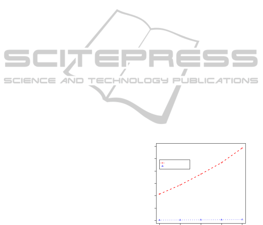
4.3 Results A: The Speed-up by
Rightward Length-maximal Flock
Patterns
In this subsection, we examine the effect of mining
of RFPs (rightward length-maximal flock patterns)
introduced in Sec. 3.2, compared to mining of FPs
(original flock patterns). For the purpose, we measure
the number of solutions and the running time by run-
ning RFPM (BFPM R, in plots) of Sec. 3.2 for min-
ing all RFPs with length ≥ k, compared to basic FPM
(BFPM) of Sec. 3.1 for mining all FPs with length
≥ k.
4.3.1 Exp 1a
In Fig. 2, we show the running time and the number of
patterns of by varying the number of points of input
size n from 60 to 100 trajectories.
Num of Points * 100
Running Time (sec)
1074
1074
1074
1074
1074
120 140 160 180 200
0 10 20 30 40 50 60
6
6
6
6
6
BFPM EXACTLEN
BFPM R MINLEN
Figure 2: Exp 1a: The running time (and the number of
patterns by mark) by algorithms FPM (BFPM) for FPs and
RFPM (BFPM R) for RFPs by varying the the total number
n of input points from 12K to 20K points, where a number
attached to each mark indicates the number of solutions.
4.3.2 Exp 2a
In Fig. 3, we show the running time by varying the
length of input trajectory database from 100 to 200
TrajectoryPatternMininginPractice-AlgorithmsforMiningFlockPatternsfromTrajectories
149
Length of DB * 100
Running Time (sec)
474
594
714
834
954
1074
1 1.2 1.4 1.6 1.8 2
0 30 60 90 120 160 200
6
6
6
6
6
6
BFPM EXACTLEN
BFPM R MINLEN
Figure 3: Exp 2a: The running time (and the number of
patterns by mark) by algorithm FPM (BFPM) for FPs and
RFPM (BFPM R) for RFPs varying the length T of input tra-
jectories from 100 to 200 points, where a number attached
to each mark indicates the number of solutions.
trajectories.
From Exp 1b and Exp 2 above, we see that the
algorithm RFPM exactly detect the number K = 6 of
true patterns, while FPM detects the larger numbers
depending on n.
4.3.3 Summary of Results A
Overall, RFPM with RFPs is around 50 times faster
than FPM with FPs as well as the number of RFPs is
around 100 times smaller than that of FPs at maxi-
mum in our experiments.
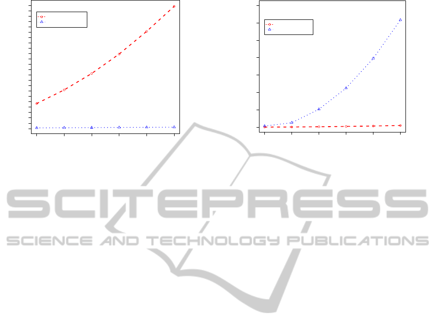
4.4 Results B: The Speed-up by
Geometric Database Reduction
In this subsection, we examine the speed-up by ge-
ometric database reduction technique introduced in
Sec. 3.3. The task is mining all RFPs in a database.
We compared two algorithms RFPM (BFPM R, in
plots) of Sec. 3.1 and G-RFPM (GFPM R, in plots) of
Sec. 3.3, without and with geometric database reduc-
tion, respectively. Note that the numbers of solutions
are same between two algorithms since they solve the
same task.
4.4.1 Exp 1b
In Fig. 4, we show the running time and the number of
patterns by varying the number n of input points from
20K to 200K points, where T = 200. For example,
in the case of the input with 200K points, the running
times for RFPM and G-RFPM are 61.61 (sec) and 0.96
(sec), respectively, resulting around 70 times speed-
up.
Num of Points * 100
Running Time (sec)
6
6
6
6
6
6
200 560 920 1280 1640 2000
0 10 20 30 40 50 60 70
6
6
6
6
6
6
GFPM R MINLEN
BFPM R MINLEN
Figure 4: Exp 1b: The running time (and the number of
patterns by mark) by algorithms RFPM (BFPM R) and G-
RFPM (GFPM R) for RFPs by varying the the total number
n of input points from 20K to 200K points.
4.4.2 Summary of Results B
Overall, in the task of mining RFPs, the modified al-
gorithm G-RFPM with geometric database reduction
improves the performance of RFPM more than ten to
70 times on the basic algorithm FPM.
4.4.3 Summary of Results A and B
From Fig. 2 of Exp 1a and Fig. 4 of Exp 1b, in the case
of the input with 200K points (small dataset), the run-
ning times for FPM, RFPM, and G-RFPM are 61.61,
0.96, 0.03 (sec), respectively. From these timing, the
speed-ups from FPM to RFPM and RFPM to G-RFPM
were around 64 times and 32 times. Overall, we ob-
tained the total speed-up of around 2,000 times from
the basic FPM to most advanced G-RFPM.
5 CONCLUSIONS
In this paper, we showed empirical study of the tra-
jectory mining algorithm FPM based on the pattern-
growth approach (Pei et al., 2004). We implemented
two improvements of FPM. The experiments demon-
strated that these improved algorithms achieved order
of magnitude speed-up on artificial data sets.
REFERENCES
Arimura, H., Geng, X., and Uno, T. (2013). Efficient min-
ing of length-maximal flock patterns from large trajec-
tory data. Manuscript, DCS, IST, Hokkaido Univer-
sity. http://www-ikn.ist.hokudai.ac.jp/
∼
arim/papers/
flockpattern201303.pdf.
KDIR2013-InternationalConferenceonKnowledgeDiscoveryandInformationRetrieval
150

Avis, D. and Fukuda, K. (1993). Reverse search for enu-
meration. Discrete Applied Math., 65:21–46.
Benkert, M., Gudmundsson, J., Hubner, F., and Wolle, T.
(2008). Reporting flock patterns. Computational Ge-
ometry, 41:111–125.
Giannotti, F., Nanni, M., Pinelli, F., and Pedreschi, D.
(2007). Trajectory pattern mining. In Proc. KDD’07,
pages 330–339. ACM.
Gudmundsson, J. and van Kreveld, M. (2006). Comput-
ing longest duration flocks in trajectory data. In
Proc. ACM GIS ’06, pages 35–42. ACM.
Laube, P., van Kreveld, M., and Imfeld, S. (2005). Find-
ing REMO — detecting relative motion patterns in
geospatial lifelines. In Spatial Data Handling, pages
201–215.
Pei, J., Han, J., Mortazavi-Asl, B., Wang, J., Pinto, H.,
Chen, Q., Dayal, U., and Hsu, M.-C. (2004). Mining
sequential patterns by pattern-growth: The prefixspan
approach. IEEE TKDE, 16(11):1424–1440.
Romero, A. O. C. (March 2011). Mining moving flock pat-
terns in large spatio-temporal datasets using a frequent
pattern mining approach. Msc. Thesis, U. Twente.
Uno, T., Asai, T., Uchida, Y., and Arimura, H. (2004). An
efficient algorithm for enumerating closed patterns in
transaction databases. In Proc. DS’04, LNCS 3245,
pages 16–31.
Vieira, M. R., Bakalov, P., and Tsotras, V. J. (2009). On-line
discovery of flock patterns in spatio-temporal data. In
Proc. GIS’09, pages 286–295. ACM.
Zaki, M. J. (2000). Scalable algorithms for association min-
ing. IEEE Transactions on Knowledge and Data En-
gineering, 12(3):372–390.
Zaki, M. J. and Hsiao, C.-J. (2005). Efficient algorithms
for mining closed itemsets and their lattice structure.
IEEE TKDE, 17(4):462–478.
TrajectoryPatternMininginPractice-AlgorithmsforMiningFlockPatternsfromTrajectories
151
