
A Multiple Instance Learning Approach to
Image Annotation with Saliency Map
Tran Phuong Nhung
1
, Cam-Tu Nguyen
2
, Jinhee Chun
1
, Ha Vu Le
3
and Takeshi Tokuyama
1
1
Graduate School of Information Sciences, Tohoku University, Sendai, Japan
2
National Key Laboratory for Novel Software Technology, Nanjing University, Nanjing, China
3
VNU University of Engineering and Technology, Hanoi, Vietnam
Keywords:
Visual Saliency, Image Annotation, Multiple Instance Learning.
Abstract:
This paper presents a novel approach to image annotation based on multi-instance learning (MIL) and saliency
map. Image Annotation is an automatic process of assigning labels to images so as to obtain semantic retrieval
of images. This problem is often ambiguous as a label is given to the whole image while it may only cor-
responds to a small region in the image. As a result, MIL methods are suitable solutions to resolve the
ambiguities during learning. On the other hand, saliency detection aims at detecting foreground/background
regions in images. Once we obtain this information, labels and image regions can be aligned better, i.e., fore-
ground labels (background labels) are more sensitive to foreground areas (background areas). Our proposed
method, which is based on an ensemble of MIL classifiers from two views (background/foreground), improves
annotation performance in comparison to baseline methods that do not exploit saliency information.
1 INTRODUCTION
Image annotation is an automatic process of finding
appropriate semantic labels for images from a prede-
fined vocabulary. In other words, an image is assigned
with a few relevant text keywords that reflect the im-
age’s visual content. Image annotation has become
a prominent research topic in the domain of medical
image interpretation, computer vision and semantic
scene classification. In particular, it is useful towards
image retrieval as annotated keywords greatly narrow
the semantic gap between low level (visual) features
and high level semantics.
Automatic image annotation is a challenging task
due to various imaging conditions, complex and hard-
to-describe objects, as well as a highly textured back-
ground (Qi and Han, 2007). Unlike object recog-
nition, image annotation is a “weak labeling” prob-
lem. That means a label is assigned to the whole im-
age without any alignment of regions and the label
(Carneiro et al., 2007). As a result, the multi-instance
approach (Zhou and Zhang, 2007) is a natural solu-
tion to resolve the ambiguities in training data. Un-
like traditional supervised learning, an example (e.g.
an image) in MIL is not described by a feature vector
(a single instance) but a set of feature vectors (a bag
of instances). By considering an image as an exam-
ple and its instances as feature vectors extracted from
subregions of the image, the problem of image anno-
tation naturally fits the multi-instance setting. There
were several studies (Carneiro et al., 2007; Nguyen
et al., 2010; Yang et al., 2006) that have successfully
applied MIL to the problem of image annotation. One
disadvantage of those methods is that they treated in-
stances (sub-regions in images) equally for every la-
bel. Our observation is that we can weight instances
differently with respect to different labels. An ex-
ample is given in Figure 1, the instance (feature vec-
tor) that falls into the salient region is more relevant
the foreground object (polar bear), while the other in-
stances (background regions) are more important to-
wards the background label (snow). Even though we
do not really have the correspondence between the in-
stances (regions) and the labels (polar bear, snow) due
to the “weak labeling” problem, the observation can
be useful towards reducing noises in learning an im-
age annotation system.
In order to apply the above idea, there are several
questions that need to be addressed. The first ques-
tion is how to obtain visual saliency for image annota-
tion. Fortunately, this problem has been well studied
in computer vision (Hou et al., 2012) where the main
assumption is that “the image energy focuses on the
locations of a spatially sparse foreground, relative to a
152
Phuong Nhung T., Nguyen C., Chun J., Le H. and Tokuyama T..
A Multiple Instance Learning Approach to Image Annotation with Saliency Map.
DOI: 10.5220/0004543901520159
In Proceedings of the International Conference on Knowledge Discovery and Information Retrieval and the International Conference on Knowledge
Management and Information Sharing (KDIR-2013), pages 152-159
ISBN: 978-989-8565-75-4
Copyright
c
2013 SCITEPRESS (Science and Technology Publications, Lda.)
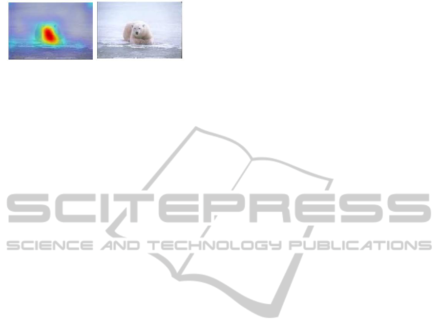
Figure 1: An example image from Corel5K data set with its
detected saliency map.
spectrally sparse background”. The second question
is that given a set of labels, how can we know a la-
bel is a foreground label or background label without
additional information from humans. Our approach
is that we let the training data decide. More specifi-
cally, we firstly obtain two kinds of learners from two
different views (background instances/foreground in-
stances). Next, we base on the performances on the
training data to decide the weights, and then combine
two kind of learners to obtain the final learner for an-
notation. To the best of our knowledge, this is the first
attempt that exploits saliency map for image annota-
tion. Experimental results show the effectiveness of
our proposed method.
The rest of the paper is organized as follows. Sec-
tion 2 reviews related works. Section 3 and 4 describe
the fundamental introduction to two building theories
(MIL and visual saliency detection) in our approach.
Section 5 introduces the proposed image annotation
approach based on MIL and visual saliency. Section
6 reports and discusses the experimental results. Sec-
tion 7 summarizes the main idea of the paper and con-
cludes some remarks.
2 RELATED WORKS
Image annotation is a typical Multi-instance Multi-
label problem (MIML) (Zhou and Zhang, 2007)
where an image is represented by a set of regions
(instances) and assigned with multiple labels. The
most successful method is based on propagating la-
bels from the nearest neighbors in the training data
(Lavrenko et al., 2003; Guillaumin et al., 2009). The
methods, however, degenerate the task of image an-
notation from a MIML problem into a set of single-
instance multi-label (SIML) problems; thus, they do
not explicitly cope with noises in training process. Al-
though the propagation approach is simple, the anno-
tation time increases linearly with the size of the train-
ing data set.
Another approach is to degenerate the image an-
notation problem into a set of multi-instance single-
label problems. Considering one specific label, we
build a classifier that determines whether to assign a
given label to an image. This classification problem
is a multi-instance problem as a label (e.g. tiger) is
assigned to an image but only relevant to some subre-
gions of the image (the other subregions are relevant
to other labels such as “forest”, “tree”). The MIL
approach explicitly takes into account these noises
in training. In the following, we will follow the
terminologies in MIL and respectively refer to “in-
stance” and “bag” as a feature vector correspond-
ing to a subregion of an image and the image it-
self. MISVM and miSVM algorithms (Andrews et al.,
2002) were adapted from single-instance learning ver-
sion of SVM in order to cope with multiple instance
data version. On the other hand, Yang et al. in-
troduced Asymmetric SVM (ASVM) to pose differ-
ent asymmetrical loss function to two types of errors
(false positive and false negative) in order to improve
the accuracy of annotation process (Yang et al., 2006).
In addition, Supervised Multi-class Labeling (SML)
(Carneiro et al., 2007) is based on MIL and density es-
timation in order to measure the conditional distribu-
tion of feature given a specific word. SML uses a bag
of image examples annotated by a particular word and
estimate the distribution of image features extracted
from the bag of images. The distribution is fitted by
mixture Gaussian distribution in a hierarchical man-
ner. SML does not consider the negative examples
in the learning binary examples. Since SML only
uses positive examples for each concept in training,
the training complexity is reduced considerably. On
another attempt, CMLMI (Nguyen et al., 2011) pro-
posed a cascade of multi-level multi-instance classi-
fiers to reduce class imbalance in MIL, and exploited
multiple modalities to improve image annotation. In
this paper, we propose an approach to image anno-
tation that uses saliency information (visual saliency
map). Our main idea is that the salient regions are
more important towards assigning foreground labels
to images.
Visual saliency detection has attracted a lot of in-
terest in computer vision as it provides fast solutions
to several complex processing. There are many stud-
ies (Ueli et al., 2004) (Navalpakkam and Itti, 2006)
that show the effectiveness of visual saliency map for
object recognition, tracking and detection. To the our
best knowledge, however, such kind of information
has not been used for image annotation before. This
paper shows that incorporating visual saliency infor-
mation to image annotation can reduce the noises as-
sociated with “weak labeling” problem, thus improve
the performance annotation process. We demonstrate
our method with miSVM, the multi-instance version
of SVM, with the support of visual saliency. Thus,
in the following, we will give a brief introduction to
these methods.
AMultipleInstanceLearningApproachtoImageAnnotationwithSaliencyMap
153
3 MULTIPLE INSTANCE
LEARNING WITH miSVM
MIL is a variation of supervised learning problems
with incomplete knowledge about labels of training
examples (Zhou and Zhang, 2007). The majority of
the work in MIL is concerned with binary classifica-
tion problems, where each example has a classifica-
tion label that assigns it into one of two categories
“positive” or “negative”. The goal is to learn a model
based on the training examples that are effective in
predicting the classification labels of future examples.
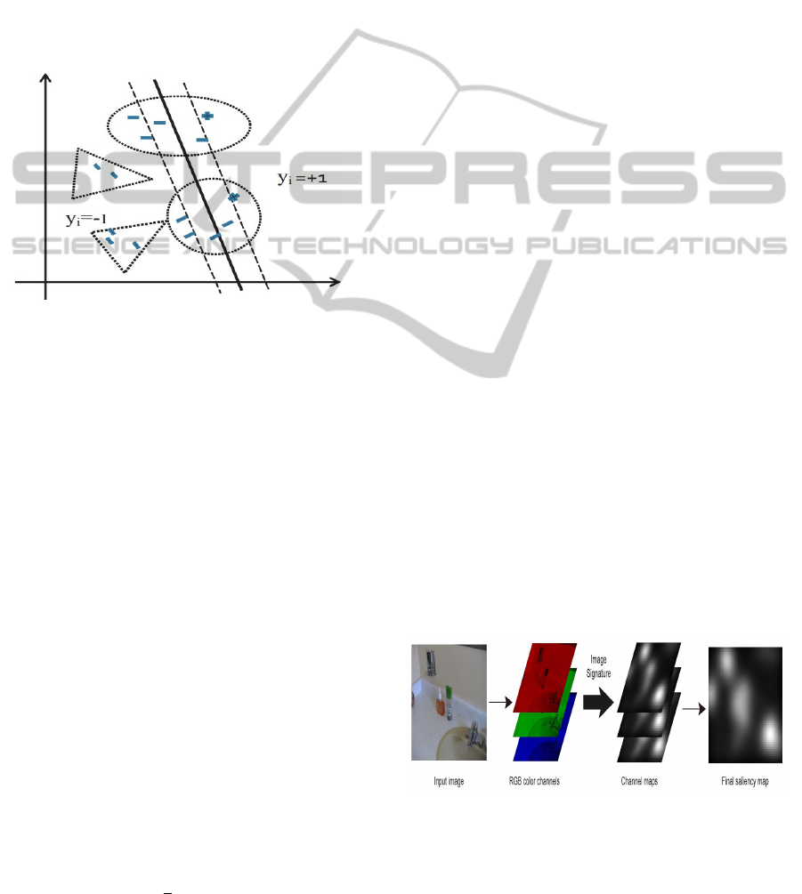
Figure 2: Multiple Instance Learning: positive and negative
bags are denoted by circles and triangles respectively.
miSVM (Andrews et al., 2002; Nguyen et al.,
2011) extends the notion of the margin from an in-
dividual instance to a set of instances (Figure 2). Let
D
y
= {(X
i
, Y
i
)|i = 1, . . . , N, X
i
= {x
j
};Y
i
= {+1, −1}}
be a set of images (bags), where a bag X
i
of instances
(x
j
) is positive (Y
i
= 1) if at least one instance x
j
∈ X
i
has its label Y
i
positive (the subregion in the image
corresponds to positive label). As shown in Figure 2,
positive bags are denoted by circles and negative bags
are marked as triangles. The relationship between in-
stance labels and bag labels can be compressed as
Y
i
= max(y
j
), j = 1, . . . , |X
i
|. The functional margin
of a bag with respect to a hyperplane is defined in
(Andrews et al., 2002) as follows:
Y
i
max
x
j
∈X
i
(ax
j
+ b)
The prediction then has the form Y
i
=
sgnmax
x
j
∈X
i
(ax
j
+ b). The margin of a positive
bag is the margin of the most positive instance,
while the margin of a negative bag is defined as the
“least negative” instance. Keeping the definition
of bag margin in mind, the Multiple Instance SVM
(miSVM) is defined as following:
minimize:
1
2
||a|| +C
N
∑
i=1
ξ
i
subject to: Y
i
max
x
j
∈X
i
(ax
j
+b) ≥ 1 −ξ
i
, i = 1, . . . , N, ξ
i
≥ 0
By introducing selector variables s
i
which denotes the
instance selected as the positive “witness” of a posi-
tive bag X
i
, Andrews et al. has derived an optimiza-
tion heuristics. The general scheme of optimization
heuristics alternates two steps: 1) for given selector
variables, train SVMs based on selected positive in-
stances and all negative ones; 2) based on current
trained SVMs, updates selector variables. The pro-
cess finishes when no change in selector variables.
4 VISUAL SALIENCY
Research of visual psychology has shown that when
observing an image, people do not have the same in-
terest in all of it. The Human Visual System (HVS)
has a remarkable ability to automatically focus on
only salient regions. Saliency at a given location is
determined by the degree of difference between that
location and its surrounds in a small neighborhood.
Thus, saliency map is obtained from summing up dif-
ferences of image pixels with their respective sur-
rounding pixels.
In this paper, we propose an approach to image an-
notation that uses salient interesting points. We use a
vector space representation of the local descriptors of
the salient regions to describe the image in an invari-
ant manner, and a classifier which is achieved based
on learning processes generates the correct annotation
for the images. In particular, for our algorithm, we se-
lect salient regions using the method which is called
“image signature” (Hou et al., 2012). It is defined
as the sign function of the Discrete Cosine Transform
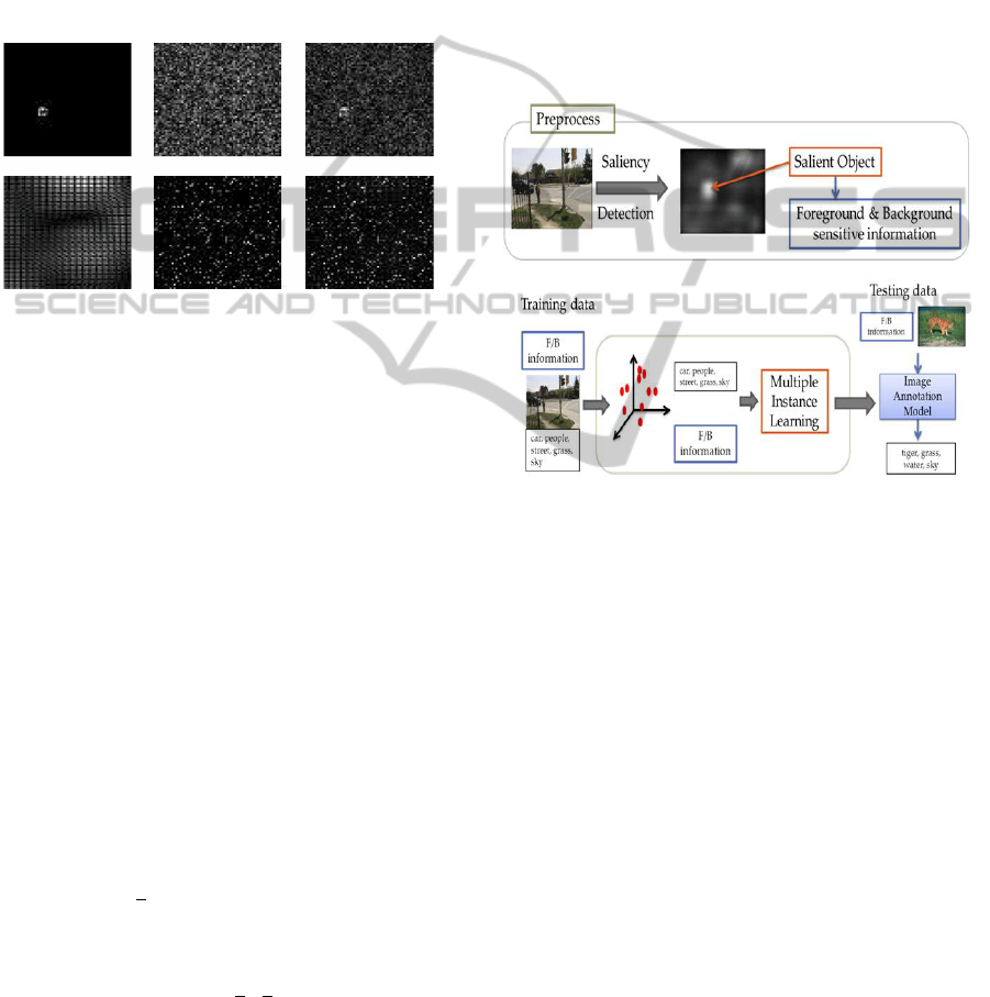
(DCT) of an image. An overview of the complete al-
gorithm is presented in the Figure 3. Firstly, the im-
age is decomposed into three channels (RGB). Then,
a saliency map is computed for each color channel in-
dependently. Finally, saliency map is simply summed
across three color channels.
Figure 3: Overview of the process of finding salient regions
(Hou et al., 2012).
Initially, they consider gray-scale images which
are presented as follows:
x = f + b (x, f , b ∈ R
N
) (1)
KDIR2013-InternationalConferenceonKnowledgeDiscoveryandInformationRetrieval
154
where, f represents the foreground and is assumed
to be sparsely supported in the standard spatial ba-
sis; b represents the background and is assumed to be
sparsely supported in the basis of DCT. That means
both f and
ˆ
b which is DCT(b) have only a small num-
ber of nonzero components in the standard spatial ba-
sis and the DCT domain respectively.
An illustration of image is standard spatial basis
and DCT is shown in Figure 4. The first row: f, b, x in
the spatial domain. The second row: the same signals
are represented in the DCT domain:
ˆ
f ,
ˆ
b, ˆx.
Figure 4: An illustration of the randomly generated images
in the spatial domain and Discrete Cosine Transform do-
main (Hou et al., 2012).
In Figure 4, f is randomly generated in the standard
spatial basis, then f is presented in DCT domain by
computing DCT(f). Since b is assumed sparsely sup-
ported in DCT domain, firstly generate DCT(b), and
then b is achieved by inversely transformed back into
spatial domain b=IDCT(DCT(b)). This idea is the
same to represent for x in spatial domain and DCT do-
main. Based on the property that f and b are sparsely
supported in different domains, they can isolate the
set of fixes for f which is nonzero.
Given an image x, the main idea of image signa-
ture algorithm is described as follows: firstly, they
separate the support of f by taking the sign of the mix-
ture signal x in the DCT domain. The purpose of this
step is to sharpen the image by keeping only the high
frequency components.
ImageSignature(x) = sign(DCT (x)) = sign( ˆx) (2)
Then, inversely transform it back into the spatial do-
main by computing the reconstructed image.
x = IDCT [sign( ˆx)] (3)
Finally, the saliency map m of an image is generated
by smoothing the squared reconstructed image.
m = g ∗ (x ◦ x) (4)
where, g is a Gaussian kernel. In this case, a Gaussian
smoothing is necessary since a salient object is not
only spatially sparse but also localized in a contiguous
region.
5 IMAGE ANNOTATION BASED
ON MIL & VISUAL SALIENCY
In this section, we formulate image annotation as a
supervised learning problem under multiple instance
learning frameworks. In order to improve the accu-
racy and efficient in image annotation, we introduce
the approach to it based on visual saliency.
5.1 Overview of proposed Model
Our model contains two processes and it is showed in
the Figure 5.
Figure 5: Overview of proposed model.
In the pre-process, we apply image signature al-
gorithm (Hou et al., 2012) to detect the salient object
of images. Based on the saliency map, we achieve the
foreground and background sensitive information of
the image. In the next step, we construct an automatic
image annotation system based on saliency map. As
mentioned earlier, we decompose the problem of im-
age annotation into a set of multi-instance single-label
problems. In other words, a MIL binary classifier is
learned in order to link a image region to a specific
keyword (e.g. tiger) , i.e. an image is assigned with
“tiger” if it is classified “positive” according to the
“tiger” MIL classifier . Then the learned classifiers
are used to produce the annotation for new input im-
ages. During learning MIL classifiers, we further re-
duce the ambiguity in image annotation by using the
saliency information as a supporting factor for MIL.
The idea is that the region is more salient is sam-
pled more for foreground labels. A simple solution
is based on sampling/weighting method. A salient re-
gion is weighted more, thus it have higher ability to
be annotated for foreground label.
AMultipleInstanceLearningApproachtoImageAnnotationwithSaliencyMap
155

5.2 Image Annotation with Foreground
and Background Decomposition
We assume that every image is divided into regions,
and each region is described by a feature vector (in-
stance). Thus, an image X
i
is presented by a set of
feature vectors X
i
= {x
i1
, x
i2
, ..., x
in
}, where n is the
number of regions in image X
i
.
Based on the saliency map which is achieved by
image signature algorithm (Hou et al., 2012), we as-
sign the saliency values to regions of one image. Note
again that we have a one-to-one correspondence be-
tween regions and instances. Supposed that m is the
saliency map, where m(l, k) represents the saliency
value of pixel (l, k) in the image, δ
i j
that a probability
of region
j
(or instance j) of image X
i
is foreground.
Therefore, δ
i j
is defined as follows:
δ
i j
=
∑
(l,k) in region r
j
m(l, k)
∑
(l
0
,k
0
) in image X
i
m(l
0
, k
0
)
(5)
Then, (1−δ
i j
) indicates the probability for region
j
of
image X
i
to be a background region.
Considering the multiple instance Support Vector
Machine (miSVM) algorithm (Andrews et al., 2002)
that work directly with the bags of instances, the
question is that how we modify the instance weights
when we have already gained foreground-sensitive
and background-sensitive information. The proposed
solution is that add more “foreground-sensitive” or
“background-sensitive” information to positive bags.
Note that we only deal with the instances in the posi-
tive bags during training since negative bags have no
ambiguous (all the instances in negative bags are neg-
ative).
For foreground enhanced bags (images with
more “foreground-sensitive” information”), we will
enforce foreground instances by adding more
foreground-sensitive “pseudo” instances. On the
other hand, for background enhanced bags, we
will enforce background instances by adding more
background-sensitive “pseudo” instances. Note that
foreground enhanced bags (background enhanced
bags) have more useful information towards fore-
ground (background) labels.
Given a maximum the number of added pseudo
instances K, and X
i
is the bag of instances/regions;
the pseudo code for adding more pseudo instance is
presented as in Algorithms 1-2.
Foreground-enhanced bag X
f
i
is enriched with
foreground-sensitive information. The probability
of instance/region c added to bag X
f
i
is estimated
based on the multinomial distribution of δ; where
δ = {δ
i1
, δ
i2
, , δ
in
} is a vector of n elements (n is num-
ber of regions), and δ
i j
( j = 1 : n) is the probability
Algorithm 1: Generating Foreground-sensitive Bag.
1: Input:
ˆ
X
i
= {X
i
, δ
i
}, K is the number of added
pseudo-instance.
2: Output: Foreground-enhanced bag X
f
i
3: Initialize X
f
i
= X
i
4: Consider the set of C instances in X
i
5: for i=1:K do
6: Sample c from Multinominal(δ
i
)
7: Add instance c to bag X
f
i
8: end for
Algorithm 2: Generating Background-sensitive Bag.
1: Input:
ˆ
X
i
= {X
i
, δ
i
}, K is the number of added
pseudo-instance.
2: Output: Background-enhanced bag X
b
i
3: Initialize X
b
i
= X
i
4: Consider the set of C instances in X
i
5: for i=1:K do
6: Sample c from Multinominal(1-δ
i
)
7: Add instance c to bag X
b
i
8: end for
of region
j
is foreground so that
∑
n
j=1
δ
i j
= 1. δ
i j
value
is calculated based on the saliency value.
Besides, background-enhanced bag X
b
i
is
enriched with background-sensitive informa-
tion. The probability of instance/region c
added to bag X
b
i
is estimated based on the
multinomial distribution of (1 − δ); where
(1 − δ) = {
1−δ
i1
∑
n
j=1
(1−δ
i j
)
,
1−δ
i2
∑
n
j=1
(1−δ
i j
)
, ...,
1−δ
in
∑
n
j=1
(1−δ
i j
)
}: is
a vector of n elements, and (1 −δ
i j
) (with j = 1, ..., n)
is the probability of region
j
is background.
Furthermore, in order to combine foreground-
sensitive and background-sensitive information at
classifier level, we will build the classifier based on
AdaBoost two-step boosting model. Assume that,
based on the foreground-sensitive and background-
sensitive information we can build two classifiers H
f
,
H
b
respectively. The final classifier of bag X
i
is the
combination of H
f
and H
b
:
H(X
i
) = λ × H
f
+ (1 − λ) × H
b
(6)
In order to automatically estimate the parameter λ, we
build classifier ensemble based on AdaBoost two-step
boosting with base learner is miSVM. The pseudo
code of AdaBoost two-step boosting is presented as
follows:
The method of combining the class predictions
from multiple classifiers is known as ensemble learn-
ing (Rokach, 2010). AdaBoost is one of the most
prominent ensemble learning algorithms. The main
idea is that AdaBoost generates multiple training sets
from the original training sets and then trains compo-
KDIR2013-InternationalConferenceonKnowledgeDiscoveryandInformationRetrieval
156

Algorithm 3: Two-Step Boosting with MIL.
1: Input:
Given a training dataset D =
{(
ˆ
X
1
, y
k1
), . . . , (
ˆ
X
d
, y
kd
)} w.r.t the label y
k
where y
ki
∈ {−1, +1} and
ˆ
X
i
= {X
i
, δ
i
};
A testing image
ˆ
X;
The number of iterations T for AdaBoost.
2: Output:
H - an ensemble classifier of 2 × T weak classi-
fiers;
The predictive value for X.
3: TRAINING:
4: Initialize D
f
= {}, D
b
= {}
5: for each positive bag X
i
in D do
6: Obtain X
f
i
, X
b
i
from
ˆ
X
i
using Algorithm 1-2.
7: D
f
= D
f
∪ X
f
i
and D
b
= D
b
∪ X
b
i
8: end for
9: Boosting 1st step: foreground-sensitive
10: [H
f
, λ
f
] ← miSVM.Adaboost(D
f
, T )
11: Boosting 2st step: background-sensitive
12: [H
b
, λ
b
] ← miSVM.Adaboost(D
b
, T )
13: TESTING:
14: Obtain X
f
and X
b
from
ˆ
X = {X, δ}.
15: Predictive value for testing image
ˆ
X
H(
ˆ
X) =
∑
T
i=1
λ
f
i
h
f
i
(X
f
) +
∑
T
i=1
λ
b
i
h
b
i
(X
b
)
∑
T
i=1
λ
f
i
+
∑
T
i=1
λ
b
i
nent learners. It focus on the misclassified from pre-
vious round. From each generated training set, Ad-
aBoost induces the ensemble of classifiers by adap-
tively changing the distribution of the training set
based on the accuracy of the previously created classi-
fiers and then use a measure of classifier performance
to weight the selection of training examples and the
voting. Initially, all weights are set equally, but on
each round, the weights of incorrectly classified ex-
amples are increased so that the weak learner is forced
to focus on the hard examples in the training set. The
predictions of the component learners are combined
via majority voting, where the class label receiving
the most number of votes is regarded as the final pre-
diction.
6 RESULTS AND DISCUSSIONS
6.1 Dataset and Experimental Settings
We use the Corel5k benchmark for the experiment
(Duygulu et al., 2002). It contains 5,000 images and
each image is segmented into 1-10 regions. The data
set is divide into two parts: training set contains 4,500
images and the rest of 500 images for testing. In ad-
dition, each image is manually annotated with 1 to
5 keywords from the vocabulary list of 371 distinct
words. Prior to modeling, every image in the data set
is pre-segmented into sub-regions using normalized
cuts algorithms (Shi and Malik, 2000). The feature set
consists of 36 features were extracted for each region:
18 color features, 12 texture features and 6 shape fea-
tures (Duygulu et al., 2002).
We implement classifier ensemble based-on Ad-
aboost with base learner is miSVM (Rokach, 2010).
We use the AdaBoost algorithm which is imple-
mented in the WEKA (Hall et al., 2009) with the num-
ber of iterations is set to 10. We compare 5 models
with base learner is miSVM:
• Baseline_miSVM: baseline model;
• AdaBoost_miSVM: classifier ensemble based on
Adaboost;
• F_AdaBoost_miSVM: classifier ensemble based
on Adaboost and boosting one step with fore-
ground sensitive;
• B_AdaBoost_miSVM: classifier ensemble based
on Adaboost and boosting one step with back-
ground sensitive;
• FB_AdaBoost_miSVM: classifier ensemble
based on Adaboost and boosting two step with
foreground and background sensitive.
The quality of automatic image annotation is also
measured through the process of retrieving the test
images with a single keyword. For each image, top
words are indexes using probabilities of those words
generated by image annotation. Given a single-word
query, the system returns all images annotated with
that word, ordered by probabilities. We limited the
number of indexed words per image; in particular, we
only obtained top 5 words per image for indexing. Re-
garding a word w, the number of correctly annotated
images is denoted as N
c
, the number of retrieved im-
ages is denoted as N
r
, and the number of truly related
images in the testing set is denoted as N
t
. The preci-
sion (P), recall (R) and F
1
are defined as follows:
P(w) =
N
c
N
r
, R(w) =
N
c
N
t
, F
1
=
2 × P × R
P + R
(7)
We select 70 mostly used keywords in vocabulary
list and perform our experiments. The precision and
recall averaged over the set of words occurring in the
test images are using for evaluating image annotation
process.
AMultipleInstanceLearningApproachtoImageAnnotationwithSaliencyMap
157
6.2 Results and Discussions
Our proposed models using foreground and
background-sensitive information in image an-
notation are compared to baseline work in order to
demonstrate that image annotation with foreground
and background decomposition outperforms other
traditional methods.
The average precision, recall and F
1
for baseline
work and our four proposed models on 70 mostly used
keywords are reported in Table 1.
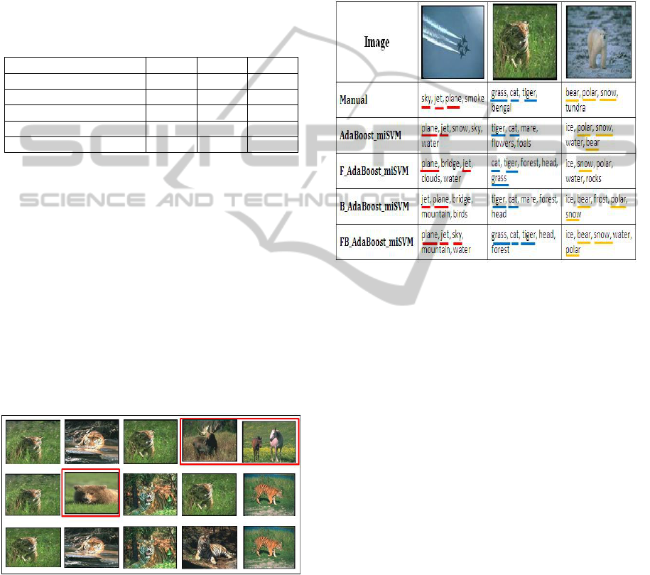
Table 1: Precision, Recall and F
1
of five models.
P R F
1
Baseline_miSVM 19.5% 37.5% 24.7%
AdaBoost_miSVM 26.7% 37.8% 30.5%
F_AdaBoost_miSVM 27.4% 37.8% 30.9%
B_AdaBoost_miSVM 25.3% 35.8% 28.6%
FB_AdaBoost_miSVM 31.9% 42.2% 36.3%
According to Table 1, it is obviously that all
of four proposed models have better results com-
pared to baseline work. Especially, the proposed
model FB_AdaBoost_miSVM has the best result in
annotation performance, which gains 31.9%, 42.2%
and 36.3% on precision, recall and F
1
value respec-
tively. Besides, the model use both foreground and
background sensitive information gain better preci-
sion, recall and F
1
value than models only use fore-
ground sensitive or background sensitive information.
Foreground-sensitive information seems useful than
background-sensitive information for image annota-
tion. It is observed that F_AdaBoost_miSVM model
has better results in terms of precision, recall and F
1
than B_AdaBoost_miSVM.
Figure 6: Top five retrieval images for query “tiger”. From
top to bottom: Baseline_miSVM, F_AdaBoost_miSVM,
FB_AdaBoost_miSVM method.
Table 1 demonstrates that our proposed meth-
ods have some improvement on baseline work via
statistical view. In Figure 6, we illustrate this im-
provement via image retrieval process. Consider-
ing top five retrieval images for query “tiger” by
using Baseline_miSVM, F_AdaBoost_miSVM and
FB_AdaBoost_miSVM model, the difference is easy
to notice. For Baseline_miSVM, two of top five
images are not correct. While one image in top
five is not exactly corresponded to the query for
F_AdaBoost_miSVM, FB_AdaBoost_miSVM suc-
cessfully retrieved all correct top five images.
In addition, Figure 7 shows the comparison of the
ground truth of sample images with their annotation
results produced by our four proposed models.
Figure 7: Comparisons of annotations made by our pro-
posed methods and annotations made by human.
In comparison to manual annotation by human, the
annotations made by our methods are significantly
reliable. In most cases, the proposed models are
able to annotate the important keywords to images
somehow accurately reflect its semantic meaning.
In addition, applying both foreground and back-
ground sensitive information give us the best re-
sults in annotation compared to model with or with-
out foreground/background sensitive information. As
you can see on three examples in Figure 7, while
the AdaBoost_miSVM, F_AdaBoost_miSVM and
B_AdaBoost_miSVM only products two correct key-
words to images, FB_AdaBoost_miSVM model pre-
cisely products three out of five keywords.
From the experimental results, we also ob-
served that labels which are considered sensitive to
background-information (e.g. water, grass, sky, coast,
etc) have performance of B_Adaboost_miSVM better
than F_Adaboost_miSVM. In order to achieve better
results, the models like B_AdaBoost_miSVM
should be more important for background-
sensitive labels. On the contrary, the key-
words like tiger, bear, horses and so on are
foreground-sensitive labels (F_Adaboost_miSVM
is better than B_AdaBoost_miSVM). Models
like F_AdaBoost_miSVM should be used in
KDIR2013-InternationalConferenceonKnowledgeDiscoveryandInformationRetrieval
158

this case. However, if there is no informa-
tion about foreground/background labels, the
FB_Adaboost_miSVM is the most suitable method
as it will automatically estimate the weights of
foreground/background information in learning the
ensemble classifier.
7 CONCLUSIONS
In this paper, we have presented a novel approach
for image annotation with the foreground and back-
ground decomposition on the view of multiple in-
stance learning. This study is to make use of saliency
map to reduce the ambiguity in multiple instance
learning for image annotation. Therefore, a simple
method based on sampling/weighting method is con-
sidered. The main idea is that the salient objects have
higher probability to be foreground.
The empirical results in this paper show that ap-
plying the foreground and background decomposition
to image annotation can yield good performance in
most cases. This provides a very simple and efficient
solution to weak labeling problem in image annota-
tion.
The results in this paper additionally show that
models using both foreground and background infor-
mation in image annotation outperforms models only
use foreground or background information. Besides,
it also proves that classifier ensemble based on Ad-
aBoost significantly improves the classification accu-
racy.
REFERENCES
Andrews, S., Tsochantaridis, I., and Hofmann, T. (2002).
Support vector machines for multiple-instance learn-
ing. In NIPS, pages 561–568.
Carneiro, G., Chan, A. B., Moreno, P. J., and Vasconcelos,
N. (2007). Supervised learning of semantic classes for
image annotation and retrieval. IEEE Trans. Pattern
Anal. Mach. Intell., 29(3):394–410.
Duygulu, P., Barnard, K., Freitas, J. F. G. d., and Forsyth,
D. A. (2002). Object recognition as machine trans-
lation: Learning a lexicon for a fixed image vocabu-
lary. In Proceedings of the 7th European Conference
on Computer Vision-Part IV, ECCV ’02, pages 97–
112, London, UK.
Guillaumin, M., Mensink, T., Verbeek, J., and Schmid, C.
(2009). Tagprop: Discriminative metric learning in
nearest neighbor models for image auto-annotation. In
Proceedings of the 12th International Conference on
Computer Vision (ICCV), pages 309–316.
Hall, M., Frank, E., Holmes, G., Pfahringer, B., Reutemann,
P., and Witten, I. H. (2009). The weka data mining
software: An update. In SIGKDD Explorations, vol-
ume 11.
Hou, X., Harel, J., and Koch, C. (2012). Image signature:
Highlighting sparse salient regions. IEEE Trans. Pat-
tern Anal. Mach. Intell., 34(1):194–201.
Lavrenko, V., Manmatha, R., and Jeon, J. (2003). A model
for learning the semantics of pictures. In Proccedings
of the 16th Conference on Neural Information Pro-
cessing Systems (NIPS’03). MIT Press.
Navalpakkam, V. and Itti, L. (2006). An integrated model of
top-down and bottom-up attention for optimizing de-
tection speed. In In IEEE Conference on Computer Vi-
sion and Pattern Recognition, CVPR ’06, pages 2049–
2056.
Nguyen, C.-T., Kaothanthong, N., Phan, X.-H., and
Tokuyama, T. (2010). A feature-word-topic model for
image annotation. In Proceedings of the 19th ACM
international conference on Information and knowl-
edge management, CIKM ’10, pages 1481–1484, New
York, USA. ACM.
Nguyen, C.-T., Le, H. V., and Tokuyama, T. (2011). Cas-
cade of multi-level multi-instance classifiers for image
annotation. In KDIR ’11: Proceedings of the Interna-
tional Conference on Knowledge Discovery and Infor-
mation Retrieval, pages 14–23, Paris, France.
Qi, X. and Han, Y. (2007). Incorporating multiple svms
for automatic image annotation. Pattern Recogn.,
40(2):728–741.
Rokach, L. (2010). Ensemble-based classifiers. Artif. Intell.
Rev., 33(1-2):1–39.
Shi, J. and Malik, J. (2000). Normalized cuts and image
segmentation. IEEE Trans. Pattern Anal. Mach. In-
tell., 22(8):888–905.
Ueli, R., Dirk, W., Christof, K., and Pietro, P. (2004). Is
bottom-up attention useful for object recognition. In
In IEEE Conference on Computer Vision and Pattern
Recognition, CVPR 2004, pages 37–44.
Yang, C., Dong, M., and Hua, J. (2006). Region-based
image annotation using asymmetrical support vector
machine-based multiple-instance learning. In Pro-
ceedings of the 2006 IEEE Computer Society Confer-
ence on Computer Vision and Pattern Recognition -
Volume 2, CVPR ’06, pages 2057–2063, Washington,
DC, USA. IEEE Computer Society.
Zhou, Z.-H. and Zhang, M.-L. (2007). Multi-instance multi-
label learning with application to scene classification.
In Proceedings of the 19th Conference on Neural In-
formation Processing Systems (NIPS), pages 1609–
1616. Monreal, Canada.
AMultipleInstanceLearningApproachtoImageAnnotationwithSaliencyMap
159
