
Does Ventriloquism Aftereffect Transfer across Sound Frequencies?
A Theoretical Analysis via a Neural Network Model
Elisa Magosso
1
, Filippo Cona
2
, Cristiano Cuppini
2
and Mauro Ursino
1,2
1
Health Sciences and Technologies Interdepartmental Center for Industrial Research (HST-ICIR), BioEngLab,
University of Bologna, Via Venezia 52, 47521, Cesena, Italy
2
Department of Electrical, Electronic and Information Engineering “Guglielmo Marconi”,
University of Bologna, Via Venezia 52, 47521, Cesena, Italy
Keywords: Visual-auditory Integration, Ventriloquism, Hebbian Plasticity, Aftereffect Generalization.
Abstract: When an auditory stimulus and a visual stimulus are simultaneously presented in spatial disparity, the sound
is perceived shifted toward the visual stimulus (ventriloquism effect). After adaptation to a ventriloquism
situation, enduring sound shifts are observed in the absence of the visual stimulus (ventriloquism
aftereffect). Experimental studies report discordant results as to aftereffect generalization across sound
frequencies, varying from aftereffect staying confined to the sound frequency used during the adaptation, to
aftereffect transferring across some octaves of frequency. Here, we present a model of visual-auditory
interactions, able to simulate the ventriloquism effect and to reproduce – via Hebbian plasticity rules – the
ventriloquism aftereffect. The model is suitable to investigate aftereffect generalization as the simulated
auditory neurons code both for spatial and spectral properties of the auditory stimuli. The model provides a
plausible hypothesis to interpret the discordant results in the literature, showing that different sound
intensities may produce different extents of aftereffect generalization. Model mechanisms and hypotheses
are discussed in relation to the neurophysiological and psychophysical literature.
1 INTRODUCTION
In daily life, we are typically exposed to events that
impact multiple senses simultaneously. Sensory
information of various natures is continuously
integrated in our brain to generate an unambiguous
and robust percept (Ernst and Bulthoff, 2004). How
multisensory integration is accomplished has
become a central topic in cognitive neuroscience,
but the neural bases still remain largely unclear.
A substantial part of research on multisensory
integration has focused on visual-auditory
interaction. A fascinating phenomenon occurs in
case of visual-auditory spatial discrepancy:
presenting a visual stimulus and an auditory stimulus
synchronous but in spatial disparity induces a
translocation of the sound perception towards the
visual stimulus (i.e., visual bias of sound
localization) (Welch and Warren, 1980; Bertelson
and Radeau, 1981; Recanzone, 2009). This
phenomenon is known as ventriloquism, as it can
explain the impression of a speaking puppet created
by the illusionist.
Although the effect in speech perception
probably involves also cognitive factors, several
studies have shown that visual bias of sound location
occurs also with simple and meaningless stimuli,
such as flashes and beeps (Bertelson and Radeau,
1981; Bertelson, 1998; Slutsky and Recanzone,
2001). Hence, it can be ascribed - at least partly - to
an automatic attraction of the sound toward the
visual stimulus. The general explanation for the
ventriloquism effect is that the brain combines
sensory information according to their reliability,
attributing a higher weight to vision which has better
spatial resolution than audition.
An interesting feature of the ventriloquism effect
is that it can be long-lasting. That is, a period of
exposure to a ventriloquism situation (adaptation
phase) induces the so-called ventriloquism
aftereffect: after the exposure, an auditory stimulus
presented unimodally is perceived shifted in the
direction of the preceding visual stimulus
(Recanzone, 1998). It has been proposed that
aftereffect reflects a form of rapid cortical plasticity
whereby representation of acoustical space is altered
360
Magosso E., Cona F., Cuppini C. and Ursino M..
Does Ventriloquism Aftereffect Transfer across Sound Frequencies? - A Theoretical Analysis via a Neural Network Model.
DOI: 10.5220/0004551403600369
In Proceedings of the 5th International Joint Conference on Computational Intelligence (NCTA-2013), pages 360-369
ISBN: 978-989-8565-77-8
Copyright
c
2013 SCITEPRESS (Science and Technology Publications, Lda.)
by the disparate visual experience.
The ventriloquism aftereffect has attracted the
interest of several researchers (Recanzone, 1998;
Lewald, 2002; Frissen et al., 2003; Woods et al.,
2004; Frissen et al., 2005). These studies examined
whether the aftereffect is specific to the spectral
characteristics of the auditory stimuli used in the
adaptation phase or instead it generalizes along the
frequency dimension. To this aim, a pure tone
stimulus at a specific frequency was used during the
adaptation phase (together with a spatially disparate
visual stimulus), and the magnitude of the aftereffect
was measured using tones at the same frequency as
the adaptation phase and at different frequencies.
Unfortunately, these studies have provided rather
diverging results. Specifically, in a first study
(Recanzone, 1998) human subjects were exposed to
either 750 Hz or 3 kHz tones synchronized with a
spatially disparate flash. Strong aftereffect occurred
only with tones at the same frequency as in the
adaptation phase, and no aftereffect was observed
with tones at the other frequency. Similar results
were obtained by two subsequent studies on humans
(Lewald, 2002) and on monkeys (Woods and
Recanzone, 2004) showing no or little transfer of
aftereffect between 1 kHz and 4 kHz stimuli. Hence,
the aforementioned studies indicated that the
aftereffect does not generalize over frequencies that
are two octaves apart. Contrary to these results,
other two studies reported generalization of
aftereffect not only across two-octave frequency
range (750 Hz and 3 kHz) (Frissen et al., 2003) but
even across four-octave frequency range (400 Hz
and 6.4 kHz) (Frissen et al., 2005). A possible
reason for such differences is that higher sound
intensities were used in studies reporting
generalization, compared to no generalization
studies, but this factor has not been investigated and
a clear explanation of the observed discrepancy is
still lacking. A better comprehension of aftereffect
generalization across frequencies can have important
implications as it may provide information on which
mechanisms and neuronal structures - and in
particular which auditory cortical areas - are
involved in ventriloquism. Indeed, frequency
response properties of single neurons in auditory
cortical areas may be put in relation with the extent
of aftereffect generalization across frequencies.
Neural network models are particularly suitable
to formulate hypotheses on the neural circuitry and
learning mechanisms underlying multisensory
integration and its perceptual phenomena. In the last
decades, we investigated different aspects of
organization and plasticity of multisensory
integration via neurocomputational models
(Magosso et al., 2008; Ursino et al., 2009; Magosso,
2010; Magosso et al., 2010a; Magosso et al., 2010b;
Magosso et al., 2010c; Cuppini et al., 2011; Cuppini
et al., 2012). In particular, in one recent work
(Magosso et al., 2012) we have proposed a model of
visual-auditory integration able to explain
ventriloquism effect and to reproduce – by
implementing Hebbian rules - the ventriloquism
aftereffect. However, that model considered only the
spatial features of the stimuli whereas the spectral
characteristics of the auditory stimuli were
completely neglected. Hence, it was not suitable to
investigate the generalization of aftereffect across
the frequencies, nor to assess which neural
mechanisms may explain the observed differences.
Aim of this work was to develop an advanced
version of our previous model in order to: i) mimic
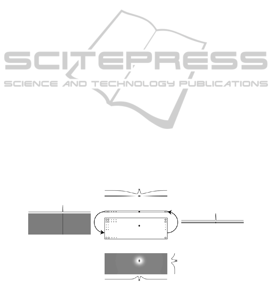
Figure 1: Network architecture. The two central rectangles represent the visual (array) and auditory (matrix) neurons. The
other panels represent the basal connections that depart from the neurons marked with the two black bullets: the lateral
panels represent inter-layer connections, while the top and bottom panels represent intra-layer connections. The darker the
colour, the more positive the connection.
DoesVentriloquismAftereffectTransferacrossSoundFrequencies?-ATheoreticalAnalysisviaaNeuralNetworkModel
361

auditory neurons coding for both spatial and spectral
properties of the stimulus; ii) reproduce
ventriloquism effect and aftereffect in these new
conditions; iii) investigate the generalization of
aftereffect across sound frequencies; iv) provide a
plausible interpretation of different extents of
aftereffect generalization.
2 METHOD
The model is an extension of our previous one
(Magosso et al., 2012), which included two one-
dimensional (1D) layers of visual and auditory
neurons, communicating via reciprocal synapses.
Each neuron in both layers coded for a particular
azimuth of the external stimulus.
In order to account for the spectral features of the
auditory stimuli, the 1D layer of auditory neurons
has been replaced by a two-dimensional (2D) matrix
(figure 1), where each neuron codes for a particular
azimuth-frequency pair of the external auditory
stimulus. The synapses have been changed
accordingly. In the new version of the model, the
visual layer has been maintained unchanged.
2.1 Model Description
The model consists of a 1D visual layer and of a 2D
auditory layer. The 1D visual layer contains N
(=
180) visual neurons. They code for the azimuth of
the external visual stimulus and are spatiotopically
aligned (proximal neurons code for proximal
positions). The 2D auditory layer contains N
x N
(= 180 x 40) auditory neurons. They code for a
particular azimuth and a particular frequency of the
external auditory stimulus, and are spatiotopically
and tonotopically aligned (proximal neurons code
for proximal positions and proximal frequencies).
Azimuths are linearly spaced by 1°, so the neurons
cover 180° along the spatial dimension; frequencies
are logarithmically spaced so the auditory neurons
cover approximately an eight-octave range along the
spectral dimension (one octave every five neurons).
Neurons within each layer communicate via lateral
intra-layer synapses, and neurons in the two layers
are reciprocally connected via inter-layer synapses.
Hence, the net input u(t) to a neuron is the sum of 3
contributions: an external input e(t); a lateral input
l(t) (from other neurons in the same layer); a cross-
modal input c(t) (from neurons in the other layer).
The activity y(t) of each neuron is computed by
passing the net input u(t) through a first order
dynamics and a steady-state sigmoidal relationship,
with the saturation level set at 1 (i.e., the activity of
each neuron is normalized to the maximum). In the
following, each of the three inputs is described. In
order to avoid border effects, the layers have a
circular structure, not shown here for briefness.
i) The External Input e(t) – The auditory external
input is reproduced as a 2D Gaussian function since
it mimics an auditory stimulus localized in space and
in frequency (tone) filtered by the receptive fields
(RFs) of the auditory neurons in the 2D space-
frequency map
e
t
E
⋅exp
ii
σ
jj
σ
(1)
E
is the stimulus intensity (arbitrary units), i and j
are the generic indices for auditory neurons along
the spatial and spectral dimensions respectively, i
and j
are the indices at which the stimulus is
centered; finally σ
and σ
define the width of the
auditory RFs along the two dimensions.
The visual external input is mimicked as a 1D
Gaussian function, representing a spatially localized
visual stimulus (e.g. a flash) filtered by the RFs of
the visual neurons in the 1D space map
e
t
E
⋅exp
ii
σ
(2)
E
is the stimulus intensity (arbitrary units), i is the
generic index for visual neurons, i
is the index at
which the stimulus is centered and σ
is related to
the width of the visual RFs along the azimuth. To
simulate the higher spatial resolution of the visual
system, σ
is assumed smaller than σ
(Magosso et
al., 2012).
ii) The Lateral Input l(t) – This input originates
from the lateral connections within each layer. For
the auditory neurons, we have
l
t
L
,
⋅
y
t
(3)
where L
,
is the synaptic strength from the pre-
synaptic auditory neuron at index hk to the post-
synaptic auditory neuron at index ij, and y
t
represents the activity of the pre-synaptic neuron.
Lateral auditory synapses are arranged according to
a 2D Mexican hat, obtained as the difference of
excitatory and inhibitory contributions each
mimicked as a 2D Gaussian function:
L
,
L
,
,
L
,
,
(4)
IJCCI2013-InternationalJointConferenceonComputationalIntelligence
362

L
,,
L
⋅exp
ih
σ
,
jk
σ
,
(5)
L
,,
L
⋅exp
ih
σ
,
jk
σ
,
(6)
In order to obtain a Mexican hat, excitation is
stronger but narrower than inhibition (L
> L
;
σ
,
< σ
,
; σ
,
< σ
,
).
For visual neurons, similar equations hold but in
1D dimension (equations in (Magosso et al., 2012));
that is lateral visual synapses are arranged according
to 1D Mexican hat (figure 1). Autoexcitation and
autoinhibition are avoided in each layer.
iii) The cross-modal input c(t) – This input
originates from the inter-layer synapses. We assume
that a visual neuron at position i sends an excitatory
synapse (W
) to all auditory neurons that code for
the same azimuth (i.e. all auditory neurons along the
i
th
column of the matrix) and receives an excitatory
synapse (W
) from any of them. Hence, the cross-
modal inputs are computed as
c
t
W
⋅
y
t
(7)
c
t
W
⋅
y
t
(8)
Parameters for the 2D auditory input, 2D lateral
auditory synapses and inter-layer synapses have
been assigned: i) to maintain a confined activation in
the auditory area preventing excessive spreading of
excitation; ii) to avoid that a unimodal stimulus
induces a phantom activation in the other non-
stimulated layer. All other parameters have been
taken from the previous paper (Magosso et al.,
2012).
2.2 Model Hebbian Rules
According to the previous paper (Magosso et al.,
2012), ventriloquism aftereffect may be explained
assuming that - during exposure to a ventriloquism
situation - lateral synapses within each layer can
change according to Hebbian learning rules
(adaptation phase).
In the present work, we adopted the same rules
as in the previous paper (Magosso et al., 2012).
Specifically, in each layer, lateral excitatory and
inhibitory synapses are subject to a potentiation
Hebbian rule with a threshold for post-synaptic
activity: excitatory synapses increase (up to a
maximum saturation level), whereas inhibitory
synapses decrease (at most down to zero) in case of
correlated pre- and post-synaptic activity, provided
that post-synaptic activity overcomes a given
threshold (assumed equal to 0.5). The maximum
saturation value for each excitatory synapsis has
been assumed equal to the maximum strength in
basal conditions (L
for the excitatory auditory
synapses). Furthermore, a normalization rule is
adopted: the sum of excitatory synapses and the sum
of inhibitory synapses entering a given neuron must
remain constant. Hence, if some of the entering
excitatory synapses increase, others decrease; if
some of the entering inhibitory synapses decrease,
others increase. All the equations of the Hebbain
synaptic rules, having 1D formulation, can be found
in our previous paper (Magosso et al., 2012).
Equations with 2D formulation, holding for the 2D
lateral auditory synapses, can be easily obtained.
Values for the learning rate were assigned so that
synapses gradually reach a new steady-state pattern
within 1000 updating steps. Simulation of an
adaptation phase consisted in exposing the network
to a spatially discrepant visual-auditory stimulation,
and maintaining the stimuli for 1000 steps during
which the lateral synapses are trained.
2.3 Evaluation of Model Performances
In psychopysical literature, ventriloquism effect and
aftereffect are assessed by measuring the
discrepancy between the perceived sound location
and the actual sound location (perceptual shift).
Hence, to evaluate model performances in response
to a stimulation, we need to compute a quantity
representing the perceived stimulus location from
the activity y(t) of all neurons within a layer. Here,
we used the barycenter metric (Magosso et al.,
2012): the perceived location is taken as the average
position (barycenter) of the layer population activity.
Hence, the perceived location of an auditory
stimulus is computed as follows
z
t
y
t
∙i
y
t
(9)
To assess network behaviour before adaptation
(basal conditions) and after adaptation, we
stimulated the network starting from the resting
condition (zero activity of all neurons). Stimuli were
maintained throughout the overall simulation until
DoesVentriloquismAftereffectTransferacrossSoundFrequencies?-ATheoreticalAnalysisviaaNeuralNetworkModel
363

the network reached a new-steady state condition, at
which the perceived stimulus location was
computed.
3 RESULTS
We first verified the ability of the modified model to
reproduce the ventriloquism effect in basal
conditions; then adaptation phases were simulated
and ventriloquism aftereffect and its generalization
across sound frequencies were investigated.
Figure 2 shows the response of the network to a
unimodal (visual or auditory) stimulation. In left
panels (a and c), a visual stimulus (with intensity E
= 15) is applied at 100°. Activation of visual neurons
assumes high values very close to the position of the
stimulus application, and declines rapidly to zero as
moving away from it. In right panels (b and d), an
auditory stimulus (with intensity E
= 20) is applied
at position 80° and at frequency 1.1 kHz. Activation
in the auditory layer assumes lower values and has a
wider extension, involving a larger number of
neurons (both along the position and frequency
dimensions). In both cases, unimodal stimulation
does not produce any phantom activity in the other
layer, which remains silent.
Figure 2: Activation for unimodal stimuli. Upper panels
show plots of the visual activations; lower panels show
maps of the acoustic activations (white = 0, black = 1).
Figure 3 shows the ventriloquism effect. A visual
stimulus at position 100° (intensity E
= 15) and an
auditory stimulus at 80° and 1.1 kHz (intensity E
=
20) are simultaneously presented to the network and
the activation of the auditory layer is displayed at
different snapshots during the simulation. Since
auditory stimulation induces a large activation,
involving also neurons at position 100°, a positive
feedback occurs between visual and auditory
neurons at that position thanks to the inter-layer
synapses (panel a). Hence, auditory neurons around
100° become rapidly very active (panel b);
moreover, they reinforce reciprocally via lateral
excitation and compete with more distant neurons
via lateral inhibition (panel c and d). At steady state
(last panel), the auditory activation is biased toward
the position of the visual stimulus, resulting in a
perceptual shift - perceived location minus actual
location - of 4°. On the contrary, the perception of
the visual stimulus exhibits a negligible shift (less
than 0.1°). These values are within the range of real
data (Bertelson and Radeau, 1981).
Figure 3: Acoustic activation at different simulation steps
(20, 40, 70, 200) during bimodal stimulation (white = 0,
black = 1).
Then, adaptation phases were simulated. In the first
adaptation phase, the same stimuli as those used in
figure 3 were delivered (visual stimulus: E
= 15 at
100°; auditory stimulus: E
= 20, at 80° and 1.1
kHz). Hence, 1.1 kHz represents the adaptation
frequency and 80° represents the adaptation position.
Results of synapses training are shown in figure
4. The figure displays the synapses – before and
after adaptation – entering two auditory neurons that
code for position 100° (the position of the visual
stimulus) and for the adaptation frequency (1.1 kHz)
(panels a and b) and the two-octave higher
frequency (4.4 kHz) (panels c and d). Synapses
targeting these two neurons exhibit similar changes
that can be summarized as follows: i) stronger
synapses are received from a wide area of neurons
left of 90° spreading across frequencies and
positions; ii) strongly reinforced synapses are
received from a strip of neurons around 100°,
covering almost all frequencies. These modifications
are due to the pattern of auditory activation during
adaptation (figure 3).
To assess the resulting aftereffect, the network
was tested unimodally by applying an auditory
stimulus at 80° (adaptation position), with intensity
1 45 90 135 180
0
0.5
1
Activation
Visual stimulation
Frequency (Hz)
Azimuth (deg)
1 45 90 135 180
275
1100
4400
1 45 90 135 180
0
0.5
1
Acoustic stimulation
Azimuth (deg)
1 45 90 135 180
275
1100
4400
c
a
d
b
Frequency (Hz)
1 45 90 135 180
275
1100
4400
1 45 90 135 180
275
1100
4400
Frequency (Hz)
Azimuth (deg)
1 45 90 135 180
275
1100
4400
Azimuth (deg)
1 45 90 135 180
275
1100
4400
c
a
d
b
IJCCI2013-InternationalJointConferenceonComputationalIntelligence
364
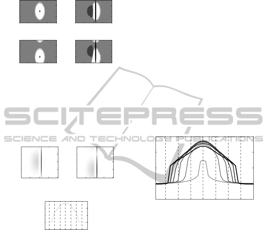
Figure 4: Synapses pre and post adaptation targeting
neuron at 100°, 1.1 kHz (upper panels), and neuron at
100°, 4.4 kHz (lower panels). The colormap is discretized
to enhance the quality of the panels. Brighter colours
denote negative (inhibitory) synapses, darker colours
denote positive (excitatory) synapses.
E
= 20, at each of the two frequencies 1.1 kHz and
4.4 kHz (figure 5, panel a and b).
Figure 5: Aftereffect. Upper panels show the auditory
activation, after training, in response to unimodal acoustic
stimulation at the adaptation frequency and two octaves
above. The lower panel shows the perceptual shift at all
the frequencies analysed (one octave per grid line).
In both cases, after adaptation, the auditory stimulus
induces an elongated area of high activation around
position 100° that spans across the frequency
dimension (that is, a large number of neurons coding
for positions close to 100° are strongly activated), in
agreement with synaptic modifications. Such
activation results in a perceptual shift (perceived
location minus actual location) equal to 2.71° for the
testing stimulus applied at 1.1 kHz and 1.38° for the
testing stimulus applied at 4.4 kHz. Finally, figure 5
panel c displays the values of the aftereffect
(perceptual shift) obtained by varying the testing
stimulus over the whole range of frequencies. We
can observe that in this case, the model exhibits a
generalization of aftereffect across more than two-
octave distance, in agreement with some
experimental data (Frissen et al., 2003; Frissen et al.,
2005).
As mentioned in the introduction, studies
reporting generalization tend to use sounds at higher
intensities than those showing no generalization.
Therefore we investigated the effects of stimulating
the network (both during the adaptation phase and
the testing phase) with an auditory stimulus at
different intensities, ranging from 17 to 23. Except
for the auditory stimulus intensity, stimulus
configurations during adaptation were the same as in
figure 3. After each adaptation phase, the perceptual
shift in sound localization (sound applied in 80°)
was tested across the whole spectral range, and was
displayed as a function of the test frequency.
Figure 6: Influence of the acoustic stimulus intensity on
the aftereffect generalization across frequencies (one
octave per grid line). Different lines represent the shifts
obtained for intensities ranging from 17 (brightest line) to
23 (darkest line).
Results for each sound intensity are reported in
figure 6. The model predicts that the pattern of
aftereffect generalization is largely influenced by the
intensity of auditory stimulus. At low sound
intensity (E
= 17), a mild aftereffect (1.5°) occurs
only at the adaptation frequency. As intensity is
increased (E
= 18), a stronger aftereffect occurs at
the adaptation frequency and aftereffect generalizes
approximately across one-octave range.
Generalization enlarges at intensity E
as high as 19;
anyway, at two-octave distance (4.4 kHz) aftereffect
is declined to zero. These two latter conditions
(intensity E
= 18 and 19) reproduce results of the
two studies (Recanzone, 1998; Lewald, 2002)
reporting no transfer of aftereffect across sounds that
Before adaptation
Frequency (Hz)
1 45 90 135 180
275
1100
4400
Frequency (Hz)
Azimuth (deg)
1 45 90 135 180
275
1100
4400
Post adaptation
1 45 90 135 180
275
1100
4400
Azimuth (deg)
1 45 90 135 180
275
1100
4400
c
a
d
b
Frequency (Hz)
Azimuth (deg)
1 45 90 135 180
275
1100
4400
Azimuth (deg)
1 45 90 135 180
275
1100
4400
275 1100 4400
-1
0
1
2
3
Aftereffect generalization
Perceptual shift (deg)
Frequency (Hz)
c
a
b
275 1100 4400
-1
0
1
2
3
Aftereffect generalization
Perceptual shift (deg)
Frequency (Hz)
DoesVentriloquismAftereffectTransferacrossSoundFrequencies?-ATheoreticalAnalysisviaaNeuralNetworkModel
365

differed by two octaves. As intensity of the auditory
stimulus further increases (E
> 19), aftereffect
transfers to a larger range of frequencies showing a
substantial value at two-octave distance – as in the
studies by Frissen et al. (Frissen et al., 2003; Frissen
et al., 2005) - and even generalizing across almost
three octaves (intensity E
> 21).
Figure 7: Reduction of aftereffect generalization for a
small acoustic intensity (E
= 17). Panel a show the
response to bimodal stimulation before adaptation. Panels
b and c show the synapses toward the neurons at 100°, 1.1
kHz and 100°, 4.4 kHz (two octaves above), after the
adaptation (colormaps are discretized as in figure 4).
Panels d and e show the activation of acoustic neurons in
response to unimodal acoustic stimuli at 1.1 kHz and 4.4
kHz (position 80°), after adaptation. For panels a, d and e
white = 0 and black = 1.
To better comprehend these differences, figure 7
displays some results in the exemplary case of
stimulus intensity as low as 17. In particular, panel a
shows the activation of the auditory area in the
ventriloquism situation in basal synapses condition
(i.e. before adaptation). The lower stimulus intensity
induces a lower activation in the auditory layer,
especially around actual sound position (compare
with figure 3 panel d). This produces some
differences in synapses training (panel b and c).
Patterns of trained synapses are similar to those
displayed in figure 4; however, the overall excitation
from the area of neurons at left of 90° (i.e., around
the adaptation position) is smaller, spreading less
across sound positions and frequencies. The reduced
synaptic reinforcement from neurons far from the
adaptation frequency - joined with the low intensity
of the testing stimulus - explains why the aftereffect
remains confined to the adaptation frequency (figure
7, panel d and e). In particular, a mild aftereffect
(1.5°) occurs only with the testing stimulus at the
adaptation frequency (panel d), while aftereffect is
completely absent for the testing stimulus at two-
octave distance (panel e).
4 CONCLUSIONS
In this work, we present a model of ventriloquism
effect and aftereffect which is a modification of a
model we previously developed (Magosso et al.,
2012). The important extension concerns the
inclusion of the spectral properties of auditory
neurons, coding not only for the azimuth of the
auditory stimulus (as in the previous paper) but also
for its frequency. This extension has important
implications since it allows the investigation of some
important aspects of ventriloquism aftereffect that
were neglected by the previous model.
Specifically, we explore generalization of
aftereffect across sound frequencies, in order to
provide a coherent interpretation of the discrepant
results presented in the literature; indeed
experimental results vary from aftereffect being
limited to the adaptation frequency (Recanzone,
1998; Lewald, 2002) to aftereffect generalizing
across two or even more octaves (Frissen et al.,
2003; Frissen et al., 2005).
Results obtained by model simulations indicate
that the intensity of the auditory stimulus used
during the adaptation and testing phase may play a
role in producing different extents of aftereffect
generalization. In particular, at small sound
intensities aftereffect remains confined close to the
adaptation frequency, whereas at higher sound
intensities it transfers across almost three octaves
(figure 6). The model ascribes these differences to
different amounts of activation in the auditory layer.
In particular: i) Small sound intensities induce
weaker and narrower activation in the auditory layer
compared to high sound intensities. ii) During
adaptation with small sound intensities, auditory
neurons at the sound position (80°), far from the
adaptation frequency, are not or little active (figure
7, panel a). Therefore, their synapses targeting other
auditory neurons at the visual stimulus position
(100°) do not reinforce sufficiently (figure 7, panel
c). Conversely, during adaptation with high sound
intensity, neurons at the sound position (80°), even
far from the adaptation frequency, are active (figure
3, panel d) and their synapses targeting neurons at
100° reinforce (figure 4, panel d). iii) When a testing
stimulus of low intensity is applied far from the
adaptation frequency, it is not able to excite neurons
b
a
c
de
1 45 90 135 180
275
1100
4400
Frequency (Hz)
1 45 90 135 180
275
1100
4400
1 45 90 135 180
275
1100
4400
Azimuth (deg)
1 45 90 135 180
275
1100
4400
Azimuth (deg)
1 45 90 135 180
275
1100
4400
IJCCI2013-InternationalJointConferenceonComputationalIntelligence
366

at 100° and no aftereffect is observed (figure 7,
panel e); this is a consequence of the insufficient
reinforcement of the synapses and of the low applied
stimulation. Vice-versa, a testing stimulus of high
intensity far from the adaptation frequency, produces
a strong activation of neurons at position 100°
(figure 5 panel b), thanks to the reinforced synapses
further advantaged by the high applied stimulation.
Of course, pattern of synaptic modifications
strongly depend on the adopted Hebbian rules. We
adopted post-gating rules with local constraint
(individual saturation) and global constraint
(normalization). These rules are biologically
plausible and were already proven to be suitable to
reproduce ventriloquism aftereffect and a number of
its properties (Magosso et al., 2012).
The model presented in this work include some
fundamental components of self-organizing maps
(Kohonen, 1982; Haykin, 1994; Kohonen, 1995).
Indeed, it encompasses a competition process
(mediated via long-range inhibition) and a
cooperation process (mediated via short-range
excitation) within each unimodal layer. Furthermore,
it includes an unsupervised training phase, during
which the network learns without any “teacher”
throughout the repeated presentation of stimuli
patterns, and extracts the main statistical properties
of the external inputs. In this work, competition,
cooperation, and adaptation drive the network to
organize itself so that it maintains a spatial
alignment across the two different sensory
representations (visual and auditory): specifically,
the auditory space map shifts to align with the
displaced visual space map. In other words, the
network - via adaptation to visual-auditory disparity
- learns to re-assign the auditory input to a different
category with respect to the pre-adaptation
condition: in this case, the input category is the input
spatial position which is signaled by the barycenter
of auditory activation. According to the model,
category re-assignment may occur even when the
auditory input presented to the network after
adaptation exhibits “altered” features with respect to
the input used during the adaptation phase,
specifically, different spectral features. Self-
organizing maps are ubiquitous in the cortex
especially in perceptual and motor areas (at different
levels of visual processing, in the auditory cortex, in
the somatosensory cortex, in the primary motor
cortex) (Rolls and Treves, 1998), and also at
linguistic and semantic levels (Kohonen and Hari,
1999). Several neurocomputational models has
investigated how the principles of self-organization
may explain the ability of pattern recognition,
category formation and plastic adaptation observed
in biological neural systems (Fukushima, 1980;
Miyake and Fukushima, 1984; Ritter, 1990;
Kohonen and Hari, 1999; Xerri, 2012).
Results obtained by the model have several
important correspondences with in vivo-data that
may support model structure and hypotheses. First
of all, studies on humans reporting aftereffect
generalization (Frissen et al., 2003; Frissen et al.,
2005) used sound intensities (70 dB and 66 dB)
higher than those used in studies reporting no
generalization (45 dB and 60 dB) (Recanzone, 1998;
Lewald, 2002). The values of the aftereffect
predicted by the model are in line with those found
in-vivo when a similar visual-auditory spatial
discrepancy (20°) was used in the adaptation phase
(Lewald, 2002; Frissen et al., 2005). Finally, when
aftereffect generalization was observed in-vivo,
aftereffect amount showed a decreasing pattern with
increasing difference between the testing and
adaptation frequency (Frissen et al., 2005), in line
with the pattern predicted by the model (figure 6).
Furthermore, the model behavior is in agreement
with the properties of neurons in some auditory
cortical areas (such as primary auditory area and
caudomedial field). These neurons show a frequency
tuning function (i.e., the preferential range of sound
frequencies at which they respond) that enlarges as
the sound intensity increases (Recanzone, 2000;
Recanzone et al., 2000), thus exhibiting sharp tuning
functions (compatible with no aftereffect
generalization) at low sound intensity and broad
tuning function (compatible with generalization) at
high sound intensity. The model suggests that these
auditory cortical areas could be the functional sites
at which visual recalibration of auditory localization
takes place.
Future developments and variations of the
presented model are required to further deepen the
comprehension of the neural basis of ventriloquism
aftereffect and of its properties. In particular,
additional analyses are required in order: i) To better
investigate the response properties of model auditory
neurons at light of the properties of real neurons.
Indeed, as highlighted above, real auditory neurons
exhibit spatial and tuning functions that modify with
stimulus intensity (Rajan et al., 1990; Recanzone,
2000; Recanzone et al., 2000; Woods et al., 2006).
Emergence of similar properties in the simulated
neurons and their relationships with network
parameters should be investigated. ii) To relate, in a
more straightforward manner, stimulus intensities in
the model with real sound levels used in
psychophysical studies. At present, indeed, a direct
DoesVentriloquismAftereffectTransferacrossSoundFrequencies?-ATheoreticalAnalysisviaaNeuralNetworkModel
367

correspondence between model stimulus intensity
and real stimulus intensity is lacking. iii) To
simulate adaptation at different spatial positions with
a fixed visual-auditory disparity. In the present
work, the adaptation phase consisted in presenting
a visual and an auditory stimulus in fixed spatial
positions. In future, the network could be trained by
presenting two cross-modal stimuli with assigned
spatial difference but variable locations (as in
experimental studies). iv) To mimic aftereffect
generalization on even wider range of frequencies
(i.e., four-octave range as reported by (Frissen et al
2005)). This would require to augment the number
of neurons in the auditory layer. v) To explore the
involvement of other potential factors (e.g. attentive
factors) in producing different aftereffect
generalizations. Focusing selective attention to
either modality (visual or auditory) during the
adaptation phase might impact the overall size of the
aftereffects (Frissen et al., 2003). Selective attention
in the model could be simulated via
facilitatory/inhibitory effects on neuron activation
and/or via increase/decrease of synaptic learning
rate.
ACKNOWLEDGEMENTS
This work has been supported by the 2007-2013
Emilia-Romagna Regional Operational Programme
of the European Regional Development Fund.
REFERENCES
Bertelson, P. and Radeau, M. (1981). Cross-modal bias
and perceptual fusion with auditory-visual spatial
discordance. Perception & Psychophysics, 29(6),
pp.578-584.
Bertelson, P. A., G. (1998). Automatic visual bias of
perceived auditory location. Psychonomic Bullettin &
Review, 5(3), pp.482-489.
Cuppini, C., Magosso, E., Rowland, B., Stein, B. and
Ursino, M. (2012). Hebbian mechanisms help explain
development of multisensory integration in the
superior colliculus: a neural network model.
Biological Cybernetics, 106(11-12), pp.691-713.
Cuppini, C., Stein, B. E., Rowland, B. A., Magosso, E.
and Ursino, M. (2011). A computational study of
multisensory maturation in the superior colliculus
(SC). Experimental Brain Research, 213(2-3), pp.341-
349.
Ernst, M. O. and Bulthoff, H. H. (2004). Merging the
senses into a robust percept. Trends in Cognitive
Sciences, 8(4), pp.162-169.
Frissen, I., Vroomen, J., De Gelder, B. and Bertelson, P.
(2003). The aftereffects of ventriloquism: are they
sound-frequency specific? Acta Psychologica, 113(3),
pp.315-327.
Frissen, I., Vroomen, J., De Gelder, B. and Bertelson, P.
(2005). The aftereffects of ventriloquism:
generalization across sound-frequencies. Acta
Psychologica, 118(1-2), pp.93-100.
Fukushima, K. (1980). Neocognitron: a self organizing
neural network model for a mechanism of pattern
recognition unaffected by shift in position. Biological
Cybernetics, 36(4), pp.193-202.
Haykin, S. (1994). Neural Networks: A Comprehensive
Foundation, New York, Macmillan College
Publishing Company.
Kohonen, T. (1982). Self-Organized Formation of
Topologically Correct Feature Maps. Biological
Cybernetics, 43, pp.59-69.
Kohonen, T. (1995). Sel-Organizing Maps, Berlin,
Springer-Verlag.
Kohonen, T. and Hari, R. (1999). Where the abstract
feature maps of the brain might come from. Trends in
Neurosciences, 22(3), pp.135-139.
Lewald, J. (2002). Rapid adaptation to auditory-visual
spatial disparity. Learning & Memory, 9(5), pp.268-
278.
Magosso, E. (2010). Integrating information from vision
and touch: a neural network modeling study. IEEE
Transactions on Information Technology in
Biomedicine, 14(3), pp.598-612.
Magosso, E., Cuppini, C., Serino, A., Di Pellegrino, G.
and Ursino, M. (2008). A theoretical study of
multisensory integration in the superior colliculus by a
neural network model. Neural Networks, 21(6),
pp.817-829.
Magosso, E., Cuppini, C. and Ursino, M. (2012). A neural
network model of ventriloquism effect and aftereffect.
PloS one, 7(8), e42503, pp.1-19.
Magosso, E., Serino, A., Di Pellegrino, G. and Ursino, M.
(2010a). Crossmodal links between vision and touch
in spatial attention: a computational modelling study.
Computational Intelligence and Neuroscience, ID
304941, pp.1-13.
Magosso, E., Ursino, M., Di Pellegrino, G., Ladavas, E.
and Serino, A. (2010b). Neural bases of peri-hand
space plasticity through tool-use: insights from a
combined computational-experimental approach.
Neuro-psychologia, 48(3), pp.812-830.
Magosso, E., Zavaglia, M., Serino, A., Di Pellegrino, G.
and Ursino, M. (2010c). Visuotactile representation of
peripersonal space: a neural network study. Neural
Computation, 22(1), pp.190-243.
Miyake, S. and Fukushima, K. (1984). A neural network
model for the mechanism of feature-extraction. A self-
organizing network with feedback inhibition.
Biological Cybernetics, 50(5), pp.377-384.
Rajan, R., Aitkin, L. M. and Irvine, D. R. (1990).
Azimuthal sensitivity of neurons in primary auditory
cortex of cats. II. Organization along frequency-band
strips. Journal of Neurophysiology, 64(3), pp.888-902.
IJCCI2013-InternationalJointConferenceonComputationalIntelligence
368

Recanzone, G. H. (1998). Rapidly induced auditory
plasticity: the ventriloquism aftereffect. Proceedings
of the National Academy of Sciences of the United
States of America, 95(3), pp.869-875.
Recanzone, G. H. (2000). Spatial processing in the
auditory cortex of the macaque monkey. Proceedings
of the National Academy of Sciences of the United
States of America, 97(22), pp.11829-11835.
Recanzone, G. H. (2009). Interactions of auditory and
visual stimuli in space and time. Hearing Research,
258(1-2), pp.89-99.
Recanzone, G. H., Guard, D. C. and Phan, M. L. (2000).
Frequency and intensity response properties of single
neurons in the auditory cortex of the behaving
macaque monkey. Journal of Neurophysiology, 83(4),
pp.2315-2331.
Ritter, H. (1990). Self-organizing maps for internal
representations. Psychological Research, 52(2-3),
pp.128-136.
Slutsky, D. A. and Recanzone, G. H. (2001). Temporal
and spatial dependency of the ventriloquism effect.
Neuroreport, 12(1), pp.7-10.
Ursino, M., Cuppini, C., Magosso, E., Serino, A. and Di
Pellegrino, G. (2009). Multisensory integration in the
superior colliculus: a neural network model. Journal
of Computational Neuroscience, 26(1), pp.55-73.
Welch, R. B. and Warren, D. H. (1980). Immediate
perceptual response to intersensory discrepancy.
Psychological Bulletin, 88(3), pp.638-667.
Woods, T. M., Lopez, S. E., Long, J. H., Rahman, J. E.
and Recanzone, G. H. (2006). Effects of stimulus
azimuth and intensity on the single-neuron activity in
the auditory cortex of the alert macaque monkey.
Journal of Neurophysiology, 96(6), pp.3323-3337.
Woods, T. M. and Recanzone, G. H. (2004). Visually
induced plasticity of auditory spatial perception in
macaques. Current Biology, 14(17), pp.1559-1564.
Xerri, C. (2012). Plasticity of cortical maps: multiple
triggers for adaptive reorganization following brain
damage and spinal cord injury. The Neuroscientist,
18(2), pp.133-148.
DoesVentriloquismAftereffectTransferacrossSoundFrequencies?-ATheoreticalAnalysisviaaNeuralNetworkModel
369
