
Easily Reprogrammable embedded Logic Control
Václav Dvořák and Petr Mikušek
Faculty of Information Technology, Brno University of Technology, Bozetechova 2, Brno, Czech Republic
Keywords: Logic Control, Multiple-output Logic Functions, Look-Up Table (LUT) Cascades.
Abstract: The paper deals with software implementation of logic-intensive control algorithms in a form of look-up
table cascades. Provided that logic control is described by multiple-output Boolean function, control output
evaluation then reduces to several table look-ups. Depending on a required speed, one or more input
variables are used for the look-ups in a single step, and the size of tables varies accordingly. Trade-offs
between performance and memory footprint are thus possible. Changes in logic control can be implemented
rapidly by reloading data into look-up tables. The presented method is thus useful for logic control
embedded in microcontroller software.
1 INTRODUCTION
Micro-controller-based systems such as automobile
engine control systems, implantable medical
devices, remote controls, appliances, office
machines etc. are ubiquitous. Reducing the size and
cost of these systems is essential. One area
susceptible to such reduction is customized logic
that frequently uses separate devices (PLAs or
FPGAs). As we will show later, logic devices can be
replaced by fast enough evaluation of Boolean
functions in software, often without additional space
requirements.
Traditional serial evaluation of Boolean
functions one at a time, e.g in programmable logic
controllers, has been done with redundant reading of
input variables. Representing logic functions by
means of binary decision diagrams (BDD) helped to
remove that redundancy and implement single-
output logic functions using a RAM and a sequencer
(Sasao et al., 2001). However, evaluation of multiple
outputs was still done serially by means of auxiliary
variables. The similar partitioning of outputs was
used even in special purpose processors (Decision
Diagram Machines, DDMs) that evaluate decision
diagrams via branching programs (Nakahara et al.,
2010a).
Parallel evaluation of Boolean functions
specified by Multi-terminal BDDs (MTBDDs) was
done on parallel branching machine (Nakahara et al.,
2010b), but with quaternary branching only. This
evaluation can be much too slow, unless we use a
number of branching machines.
In this paper we will try to avoid branching
programs and MTBDDs completely. Our approach
is based on the iterative decomposition of the given
function, one variable at a time, producing a cascade
of look-up tables (LUTs). The next step is optimal
clustering of these LUTs into larger ones. The goal
is the minimum total size of look-up tables or the
number of LUTs in a cascade (corresponding to
evaluation time from reading the input to appearance
of the output).
The main contribution of the paper is the
upgraded algorithm of iterative decomposition
(Mikušek and Dvořák, 2008) accepting a set of
incomplete Boolean functions in cube notation and
its implementation. The paper is structured as
follows. In the following Section 2 we explain
representation of logic functions in cube notation
and then the concept of simple decomposition. In
Section 3 we deal with iterative decomposition and
related software tools. The decomposition method is
applied to two sorts of examples in Section 4. The
results are commented on in Conclusions.
2 LOGIC FUNCTIONS
To begin our discussion, we define the following
terminology. A system of m Boolean functions of n
Boolean variables,
f
n
(i)
: (Z
2
)
n
Z
2
, i = 1, 2, ..., m
(1)
will be simply referred to as a multiple-output
Boolean function F
n
. We denote Z
2
= {0, 1}.
471
Dvo
ˇ
rák V. and Mikušek P..
Easily Reprogrammable embedded Logic Control.
DOI: 10.5220/0004552004710476
In Proceedings of the 10th International Conference on Informatics in Control, Automation and Robotics (ICINCO-2013), pages 471-476
ISBN: 978-989-8565-70-9
Copyright
c
2013 SCITEPRESS (Science and Technology Publications, Lda.)

Function F
n
is incomplete if it is defined only on
set X (Z
2
)
n
; (Z
2
)
n
\ X = DC is the don’t care set.
The elements in DC are input vectors that for some
reason cannot occur. Our concern will be an
incompletely specified, multiple-output function of n
Boolean variables
F
n
: X Z
, X (Z
2
)
n
, Z {0,1, }
m
.
(2)
Function F
n
is not defined on a don´t care set DC =
(Z
2
)
n
\ X. Binary output cubes b {0,1}
m
will be
alternatively coded by integer values from Z
R
= {0,
1, 2, …, R 1}, R 2
m
.
Espresso input format fr is assumed for function
f
n
(i)
; it means that each input vector belongs to the
ON-set, to the OFF-set, or to the DC-set depending
on the ternary value 1, 0, or "~" of the output. If the
function is given in Espresso format f (PLA format),
only the ON-set is specified and an extra step is
required to generate the OFF-set.
Instead of full input vectors from (Z
2
)
n
we prefer
to use a compact cube notation [Brzozowski,1997].
(n+m)-tuples are called function cubes, in which an
element of {0, , 1}
n
is called an input cube and
element of {0, ~, 1}
m
is called an output cube. The
value of symbol "" is 0 or 1, so that one cube can
cover several input vectors.
Def. 1. Compatibility relation. Two cubes c, c´
are compatible, c c´, if they are compatible
component-wise; except pairs [0,1] and [1,0], all
other component pairs are compatible.
In other words, two cubes c and c´are compatible
if and only if they have a non-empty common sub-
cube. The compatibility relation is reflexive and
symmetric.
3 DECOMPOSITION METHOD
Def. 2. Functional decomposition of function
F
n
(x
1
, x
2
, …,x
n
) = F
n
(X)
is a serial disjunctive separation of F into two
functions G and H such that
F
n
(X) = H
k+n-h
(U, G
h
(V)), (3)
where
U, V are disjunctive subsets of set X,
U V = , U V = X,
see Fig.1. Of course, we are interested only in non-
trivial decompositions when functions G and H have
strictly fewer inputs than F, i.e.
h < n, k+ n – h < n k < h < n.
(4)
In a functional decomposition, the minimization of
the value of k is important.
G
H
F
h
F
n m
U
X
V
k
n-h
Figure 1: Disjunctive decomposition of multiple output
Boolean function F of n variables.
Decomposition can be applied iteratively to a
sequence of residual functions with a decreasing
number of variables. The method to decompose
multiple-output logic functions by means of the
BDD for characteristic function [Nakahara, 2004c]
required large data structures. In this section we will
present a more efficient method of iterative
disjunctive decomposition based on notion of
blankets (Brzozowski et al., 1997) simplified for the
iterative removal of a single input variable (|U|=1).
Instead of the exact formulation of a
decomposition algorithm, we prefer to illustrate it on
a small example, an incomplete fuction F
4
in Table
1. Let us note that a set of (n+m)-tuples does not
always define a Boolean function, because it is
possible to assign conflicting output values.
Acceptable functions must satisfy the consistency
condition, which guarantees that there are no
contradictions; shortly, if two input cubes are
compatible, their corresponding output cubes must
also be compatible.
Table 1: Cube specification of function F
4
.
x1 x2 x3 x4 y1 y2
1 0 0
0 1 1
2 1 0
0 1 0
3
0 0
1 ~
4
1 1 0 ~
5
1 1 0 0 0
6
1
1 ~ 1
7
0
0 1 1 ~
For now we will select input variables for iterative
decomposition simply in a natural sequence x
1
, x
2
,
x
3
, x
4
. Optimization of variable ordering will be
discussed later on. A single variable will be removed
from the function in one decomposition step.
Starting with variable x
1
in our example, we first
create two-block blankets 2, 3, 4 for each input
variable x
2
, x
3
, x
4
:
2 = {1, 2, 3, 4, 7; 4, 5, 6, 7}
3 = {1, 2, 3, 6, 7; 1, 2, 4, 5, 6}
4 =
{
1, 2, 3, 5; 3, 4, 6, 7
}
.
(5)
ICINCO2013-10thInternationalConferenceonInformaticsinControl,AutomationandRobotics
472

Blankets consist of subsets (blocks) of cubes
denoted by line numbers from Table 1. The first
block in each blanket includes cubes which contain
“0” or “–” in place of variable x
i
, cubes in the second
block have value “1” or “–” in place of variable x
i
.
The input blanket for the subset V is then obtained as
an intersection (*) of two-block blankets (5
):
V
=
2 *
3 *
4 =
={1, 2, 3; 3, 7; 1, 2; 4; 6, 7; 5; 4, 6}.
(6)
The main task in a serial decomposition of a
function F with given sets U and V is to find a
blanket
G
by merging blocks of
V
as much as
possible. A condition for two blocks be mergeable is
given in (Brzozowski et al., 1997). We can create
mergeable classes of blocks, preferably maximal
classes with minimal cardinality that cover all the
blocks. In our example seven compatible classes in
blanket
V
can be merged to four blocks of
G1
G1
={1, 2, 3, 7; 4, 6; 6, 7; 5}, (7)
and encoded arbitrarily with two bits - G1 outputs,
see Table 2. The minimal cardinality of
G1
ensures
that parameter k in Fig. 1 is as small as possible. Let
us note that all relevant min-terms of G1 must be
covered in the cube table as well. Function G1 in our
example is specified by four cubes (7) in Table 2.
Table 2: Cube specification of function G1.
block
V
block
G1
x
2
x
3
x
4
G1
1 1, 2, 3, 1, 2, 3, 7 0 0 0 00
2 3, 7 1, 2, 3, 7 0 0 1 00
3 1, 2 1, 2, 3, 7 0 1 0 00
4 4 4, 6 0 1 1 11
5 6, 7 6, 7 1 0 1 10
6 5 5 1 1 0 01
7 4, 6 4, 6 1 1 1 11
To construct function H1, we need two more
blankets:
U
=
1 = {1, 3, 4, 5, 6, 7; 2, 3, 4 5, 6}.
U
*
G1
= {1, 3, 7; 5; 6, 7; 4, 6; 2, 3; 5; 6; 4, 6}.
(8)
The truth table of function H1 is given in Table 3.
In the 2
nd
decomposition step we could apply the
same procedure to function G1, removing variable x
2
and looking for the input blanket
V
for the subset V
= {x
3
, x
4
}, and so on. Fig.2. shows the iterative
decomposition up to the last variable x
4
. The original
function F can be implemented as a cascade of
LUTs generating functions H
i
. We call this cascade
with one variable per LUT the generic cascade. To
reduce the cascade length and thus the overall serial
access to LUTs, we can combine several consecutive
LUTs into a single LUT. For example, function F in
Fig.2 can be implemented as two LUTs, each with 8
words 2 bit wide, specified by functions G1 and H1.
Table 3: The truth table of function H1.
1
*
G1
x
1
G1 H1
1, 3, 7 0 0 0 1 1
5 0 0 1 0 0
6, 7 0 1 0 1 1
4, 6 0 1 1 0 1
2, 3 1 0 0 1 0
5 1 0 1 0 0
6 1 1 0 1
4, 6 1 1 1 0 1
H1
G1
H2
G2
H3
G3
H4
F
x
1
x
2
x
3
x
4
F = H1 (x
1
, G1)
G1= H2 (x
2
, G2)
G2 = H3 (x
3
, G3)
G3 = H4 (x
4
)
Figure 2: Disjunctive decomposition of multiple output
Boolean function F of 4 variables.
LUT cascade composed of p-input/q-output LUTs
can be implemented by storing all LUTs in one
memory. Cascaded LUTs are accessed one by one
under a supervision of a controller. Outputs from the
previous LUT and external input(s) address together
the next LUT, until the last LUT is reached. LUTs
are stored in a RAM and can be changed at will.
Even if the memory is accessed once for each LUT
in the cascade, operation is approximately ten times
faster than branching programs (Sasao et al., 2001).
The most important characteristics of logic
functions targeted for cascade implementation is
their profile. It is cardinality of blanket
Gi
along the
LUT cascade. The random functions have the profile
(the upper bound) in the shape of a mountain peak
with slope that rises as powers of 2 at the beginning
of the cascade and descending much faster as 2
k
-
powers of R at its end. E.g. the function
implemented as a case study (n = 13 inputs, m = 8
outputs, see Appendix) has had a profile
2, 4, 8, 14, 25, 41, 62, 81, 88, 103, 90, 77, 256
(9)
The log
2
of these values give the number of binary
values transferred between neighbor LUTs. To
minimize the total size of all LUTs in a cascade, it is
thus necessary
1. to minimize the values in the profile
2. to combine consecutive LUTs in an optimal way.
As regards the first option, the program tool
EasilyReprogrammableembeddedLogicControl
473
HIDET1 (Heuristic Iterative Decomposition Tool)
was developed to aid LUT cascade synthesis
(Mikušek and Dvořák, 2008). The HIDET1 made
use of iterative decomposition of multiple output fr
Boolean functions specified by cubes with the
restriction that input cubes must be disjoint and
output cubes use only binary elements 0 and 1. This
restriction has been removed in HIDET3 used at
present: don´t cares are allowed in output cubes and
input cubes may overlap (share one or more input
vectors). It also uses a variable-ordering heuristic to
order variables optimally, because the ordering of
variables may sometimes influence the profile
dramatically (Drechsler and
Becker, 1998).
Another optimization tool has been developed
for clustering of cascade LUTs, which explores all
possible groupings of n inputs, n 32. The input to
this tool is a profile of the given function obtained
by HIDET. There are three optional optimization
criteria, searching a minimum of
the memory area, regardless the number of LUT
inputs;
the product of memory area and cascade length;
the memory area when the number of LUT inputs
is the given value N or less.
4 EXPERIMENTAL RESULTS
Two types of functions have been explored: functions
specified by weight and the real-world function
implemented in MCS 51 microcontroller as a PLA.
Def. 3 The weight of function F
n
, denoted by u, is the
cardinality of set X in Def. 2, u = |X|.
Theorem 1 (Dvořák and Mikušek, 2011) Let the
function specified by weight F
n
: (Z
2
)
n
Z
R
attains
non-zero values 1, 2, …, R-1 in |X| = u binary
vectors, X (Z
2
)
n
, R u << 2
n
. Then the profile of
the function is upper-bounded by
(2, 4, 8,…, 2
h
, u+1, u+1, u+1, …,
i
R
2
, …,
1
2
R
, R)
(10)
where h = log
2
(u+1) and i = log
2
log
R
(u+1) .
It is therefore possible for these functions to
estimate the size of LUTs for the given clustering of
input variables.
Experiments have been done on benchmark
index-generating (i.e. u = R) functions with n = 10,
16 and 20 variables. Maximal optimum profiles of
these functions have been found by HIDET tool and
are given in Table 4. The optimum LUT cascades
for random index-generating functions are listed in
Table 5. The table gives memory requirements for
the cascades with only a single cell, two cells,
generic cascades with n cells, and then cascades
optimized for memory area or for memory area -
cascade length product. The fraction of memory in
% obtained when several #LUTs are used in place of
a single LUT is also given. The interesting result is
that the memory consumption has a local minimum
for #LUTs < n. The generic cascades with the finest
granularity (#LUTs = n) are not optimal in this
respect.
The biggest drop in memory area comes from
dividing a single cell into two. Further benchmark-
specific subdivision of cascades to 4-12 cells
produces some additional decrease in memory area,
but after reaching a minimum, the memory area goes
up again. This typical trend is illustrated on the
example of lrs6 benchmark with 21 input variables
in Fig. 4. Optimization for area-time product leads to
slightly shorter cascades (2 – 6 cells) and slightly
larger memory area.
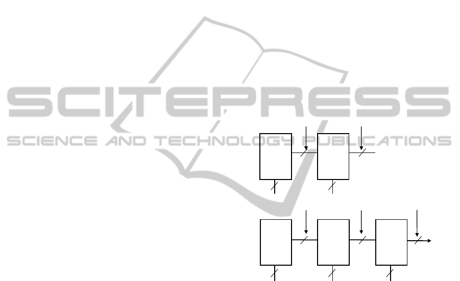
10 2
2
8 8 8
2, 4, 8, …, 256, 256, 256, 256, 256
10 3
7 8
2, 4, 8, …103, 90, 77, 256 ← profile
Figure 3: Two decompositions of PLA1 in MCS-51.
The second example has to do with LUT cascade
replacing 13-input, 8-output PLA1 in MCS-51 chip.
Here u = 175, but only logic equations are known,
see the Appendix. Equations have been converted to
PLA matrix in f format via eqntott tool and further
converted to fr format by means of Espresso
synthesizer. The resultant matrix of 147 cubes has
been processed by HIDET3 and the profile (9)
obtained. By inspection, this profile suggests 2
LUTs, first one indexed by 10 variables, the second
one by 7 outputs from the first LUT (given by |
G
| =
103) plus 3 remaining variables, Fig.3. By contrast,
had we relied on Theorem 1, then for any function of
(one more) n = 14 variables with u 256 we would
need 3 LUTs with 10, 2 and 2 input variables, all
generating 8-bit outputs, Fig.3.
ICINCO2013-10thInternationalConferenceonInformaticsinControl,AutomationandRobotics
474
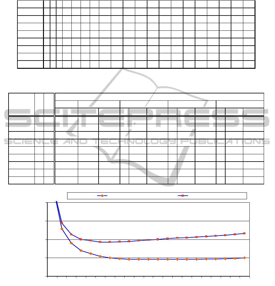
Table 4: Optimum profiles of index generating functions of 10, 16 and 20 variables and values of u as shown.
n10_u31 2 4 8 14 20 24 27 29 30 32
n10_u63 2 4 8 15 26 37 43 51 58 64
n10_u127 2 4 8 16 30 54 80 101 116 128
n16_u31 2 4 7 11 18 22 26 28 29 30 31 31 31 31 31 32
n16_u63 2 4 8 14 25 35 44 51 54 59 61 62 63 63 63 64
n16_u127 2 4 8 16 30 50 69 90 103 111 116 120 122 124 126 128
n20_u31 2 4 8 11 15 19 24 27 28 29 30 30 30 31 31 31 31 31 31 32
n20_u63 2 4 8 15 25 37 45 51 54 58 60 61 62 63 63 63 63 63 63 64
n20_u127 2 4 8 16 29 49 71 89 99 110 116 120 122 125 126 127 127 127 127 128
Table 5: Memory requirements of LUT cascades for benchmark functions with 1, 2, in, and optimum number of cells with
respect to memory area or product memory * speed (#LUTs).
#LUT=1
M [b] M [b] M [%] #L M [b] M [%] #L M [b] M [%] #L M [b] M [%]
n10_u31 10 5 5120 1920 37,50% 10 1858 36,29% 3 1600 31,25% 2 1920 37,50%
n10_u63 10 6 6144 3072 50,00% 10 3714 60,45% 2 3072 50,00% 2 3072 50,00%
n10_u127 10 7 7168 5376 75,00% 10 6914 96,46% 2 5376 75,00% 2 5376 75,00%
n16_u31 16 5 327680 15360 4,69% 16 3778 1,15% 6 3520 1,07% 4 4480 1,37%
n16_u63 16 6 393216 24576 6,25% 16 8322 2,12% 5 7680 1,95% 4 9216 2,34%
n16_u127 16 7 458752 43008 9,38% 16 17666 3,85% 5 16128 3,52% 3 21504 4,69%
n20_u31 20 5 5242880 61440 1,17% 20 4866 0,09% 8 4608 0,09% 5 6400 0,12%
n20_u63 20 6 6291456 98304 1,56% 20 11394 0,18% 7 10752 0,17% 5 13824 0,22%
n20_u127 20 7 7340032 172032 2,34% 20 24834 0,34% 7 23296 0,32% 5 28672 0,39%
memory memory * speed#LUT=in
total LUT memory in bits, % of a single LUT
#LUT=2
name in out
lrs6
1,0E+02
1,0E+03
1,0E+04
1,0E+05
1,0E+06
1 2 3 4 5 6 7 8 9 101112131415161718192021
#LUT
Mem, Mem x Length
Mem Mem x Length
Figure 4: Memory area and memory area times cascade length vs the number of LUTs.
5 CONCLUSIONS
The decomposition technique based on blankets
has been found quite suitable for engineering
applications, such as designing application-specific
systems. It has been successfully applied to
random functions specified by weight, for which
the size of the LUT cascade is computable
beforehand, and to PLA1 used in microcontroller
MCS 51. Output vectors are computable by few
accesses to LUTs.
The HIDET3 tool used for decomposition has
no restrictions on input functions; scalability is at
present limited to functions with around 20 input
variables, but the work on extending this range is
in progress. One way to reduce complexity is
EasilyReprogrammableembeddedLogicControl
475

partitioning of binary outputs and parallel
execution of resulting LUT cascades. The future
research should address this issue as well as
optimal packing of LUTs into memory when the
number of LUT inputs varies.
ACKNOWLEDGEMENTS
This research has been carried out under the
financial support of the research grants "Natural
Computing on Unconventional Platforms", GAČR
GP103/10/1517, and "Security-Oriented Research
in Information Technology", the research plan
MSM0021630528.
REFERENCES
Brzozowski, J. A., Luba, T.: Decomposition of Boolean
Functions Specified by Cubes. Research report CS-
97-01, University of Waterloo, Canada, p.36, 1997.
Drechsler, R., Becker, B. Binary Decision Diagrams -
Theory and Implementation. Springer, 1998.
Dvořák, V., Mikušek, P. (2011). On the cascade
realization of sparse logic functions, In: Proc. of the
14th EUROMICRO Conf. on Digital System Design
DSD 2011, pp. 21-28, IEEE CS, Oulu, FI.
Mikušek, P. and Dvořák, V. (2008). On Lookup Table
Cascade-Based Realizations of Arbiters, Proc. of the
11th EUROMICRO Conf. on Digital System Design
DSD 2008, pp. 795-802, IEEE CS, Parma, IT.
Nakahara, H., Sasao, T., and Matsuura, M. (2010a). A
comparison of architectures for various decision
diagram machines, International Symposium on
Multiple-Valued Logic ISMVL 2001, pp. 229-234.
IEEE CS, Barcelona, Spain,
Nakahara, H., Sasao, T., Matsuura, M., and Kawamura,
Y. (2010b). A parallel branching program machine
for sequential circuits: Implementation and
evaluation, IEICE Transactions on Information and
Systems, Vol. E93-D, No. 8, pp. 2048-2058.
Nakahara, H., Sasao. (2004c). A method to decompose
multiple-output logic functions, 41st Design
Automation Conference DAC 2004, pp. 428-433,
IEEE, San Diego, CA.
Sasao, T., Matsuura, M., and Iguchi,Y. (2001). A
cascade realization of multiple-output function for
reconfigurable hardware, International Workshop
on Logic and Synthesis IWLS01, pp.225-230. Lake
Tahoe, CA, June 12-15, 2001.
APPENDIX
Description of PLA1 in MCS-51:
INORDER = A B C D E F G H I J K L M ;
SO = !A !G !I J M | A !B !I J M | A F !I M;
CS = !A !B D !E !F !G !H !I !K !L M | A B !E !F !G !H !I !J !K !L
!M | !A !E !I M | !E !I J M | !D !I M ;
BL = !B E !F !G !H !I !J !K !L | !B C !D !H !I !J M | !B D E !H !I !J
!M | !D !I !J K M | !A !G !I J M | E H !I !L M | C !D G !I M | !A F !I
M | G !I K M | E G !I M ;
NL = !B E !F !G !H !I !J !K !L | C !D !H !I L M | !D !I !J K M | !A
!G !I J M | D E !H !I M | !A F !I M | E !I !L M | G !I K M;
V1 = !A !G !I J M | C !D F !I M | A !B !I J M | !A F !I M | F !I K M |
E F !I M ;
V3 = !B !C !D E !F !G !H !I !J !K !L | !B !G !I J K M | !D !I !J K M |
B C !I K M ;
V4 = !B C !D E !F !G !H !I !J !K !L | !B D E !F !G !H I !J !K !L M |
!A !G !I J L M | C !D !H !I L M | !A F !I L M | C !D H !I M | D E !I
L M ;
V5 = !B D E !F !G !H I !J !K !L M | !B E !F !G !H !I !J !K !L | C !D
!H !I L M | !D !I !J K M | !A !G !I J M | C !D H !I M | A !B !I J M |
D E !I L M | !A F !I M | E !I !L M .
ICINCO2013-10thInternationalConferenceonInformaticsinControl,AutomationandRobotics
476
