Bayesian versus Neural Network Analysis of Algae Data Population

A New Method to Predict and Analyse Cause and Effect

Jen J. Lee

, Jorge A. Achcar

, Emílio A. C. Barros

and Carlos D. Maciel

Signal Processing Laboratory, University of São Paulo (USP), São Carlos, Brazil

Social Medicine Department, University of São Paulo (USP), Ribeirão Preto, Brazil

Statistics Department, Maringá State University (UEM), Maringá, Brazil

Keywords: Algae, Bayes, Neural Network, Population, Machine Learning.

Abstract: In biology, advanced modelling techniques are needed since there is a mixture of qualitative, linguistics and

numerical data on the environmental and biological relationships. Also, experiments and data collecting are

expensive and time consuming, so determine which variables are relevant and using inference models less

data demanding are highly desirable. In this work, from a set of 200 multivariate data samples of algae

population and environmental variables, we propose a Bayesian method to predict compositional population

distribution. This is a good application example, since measuring environmental variables are easier to

automate, faster and less expensive than population counting that usually involves the need of a large

amount of specialized human interaction. An additive log-ratio transformation and a regression model were

applied to the data and 255.000 Gibbs samples were simulated using the OPENBUGS software. Also an

Artificial Neural Network (ANN) was designed on Matlab to predict the distribution for benchmarking

purposes. Both models showed similar prediction performance, but on the Bayesian model an analysis of

credible interval of the variables corresponding to the each regression parameters is possible, showing that

most of the variables on this study are relevant, which is consistent to the expected results in this case.

1 INTRODUCTION

The geographic region, anthropomorphic impacts

but mainly hydrology, gives to aquatic environments

great heterogeneity, especially regarding to the

concentrations of nutrients and abundance of

organisms (López-Flores et al., 2011).

Currently, it's clear that subtle variations in

nutrient levels and chemical balance from farming

land run-off and waste from sewage treatment have

serious effects, even if indirect, in the state of rivers,

lakes and even the ocean. The summers of temperate

climates around the world are characterized by

numerous reports of seasonal algal overgrowth,

resulting in poor water clarity, massive deaths of fish

from reduced oxygen levels and the closure of

recreational water facilities because of toxic effects

from algae (Univesity of California - Irvine, 1999).

However, algae, when maintained in controlled

processes, can be used for carbon sequestration,

production of biomass, oils, compounds of interest

for the industry and act as biological indicators, such

as diatoms, that have a high sensitivity in small

changes in acidity of its environment.

The need to reduce human impact on our waters

and make use of algae on controllable processes has

stimulated numerous researches, mainly in the field

of biology with the goal of identifying the crucial

variables for chemical control in biological

processes. That said, the relationship between

chemical and biological characteristics is complex

and the need for advanced modeling techniques is

expected, especially when using data containing, in

addition to the great number of variables, the

mixture of qualitative (fuzzy), linguistic and

numerical information. It is important to note that, in

biological processes, conducting experiments and/or

collecting samples probably has a great cost of time

and resources to be made and samples are often

incomplete or inconsistent, therefore, little data may

be available, affecting inference methods and

analysis that are based solely on a large amount of

data.

Regardless of the approach one takes to statistics,

the process of statistics involves (1) formulating a

research question, (2) collecting data, (3) developing

a probability model for the data, (4) estimating the

482

J. Lee J., A. Achcar J., A. C. Barros E. and D. Maciel C..

Bayesian versus Neural Network Analysis of Algae Data Population - A New Method to Predict and Analyse Cause and Effect.

DOI: 10.5220/0004552304820488

In Proceedings of the 5th International Joint Conference on Computational Intelligence (NCTA-2013), pages 482-488

ISBN: 978-989-8565-77-8

 2013 SCITEPRESS (Science and Technology Publications, Lda.)

model, and (5) summarizing the results in an

appropriate fashion to answer the research question

(a process often called “statistical inference”)

(Lynch, 2007).

At this work we suggest the use of a Bayesian

model for multivariate compositional processing of

data collected in European rivers to create a model

for inference of population distribution of algae that

have quantitative (concentrations of chemical

compounds, pH, etc.) and qualitative (season, etc.)

variables. We also propose a method to identify the

variables that cause the most significant effects on

this population distribution. The performance of

Bayesian inference model was also compared to an

Artificial Neural Network.

On section 2 we describe the data and the pre-

processing method used to prepare the variables and

the compositional data to analysis, on section 3 the

Bayesian model is described and the results of this

analysis are presented, on section 4 the Artificial

Neural Network design is described and on section 5

there is a comparison of performance between the

two prediction models, finally on section 6 the

conclusions are discussed.

2 DATA SAMPLES

The data used in this paper are the results of a

research on river water quality, where samples were

taken from different European rivers over a period

of approximately one year. These samples were

analyzed for several variables as nitrogen in the

form of nitrates, nitrites and ammonium, phosphates,

pH, oxygen, chloride. In parallel, algae population

distributions from these samples were determined.

Although chemical analysis is relatively inexpensive

and easily automated, biological analysis involves

the examination under a microscope, requiring

trained manpower and is usually expensive and very

slow.

The data set contains 200 samples, where the

first 11 values are: season of the year (winter,

spring, autumn or summer), river size (small,

medium or large), water speed (low, medium or

high) and 8 chemical concentrations (according to

Table 1). These variables are known to be relevant

to the algae species population distribution.

The last 7 columns represent the distribution of

different types of algae (according to Table 2), and

these do not represent the entire population of algae

in the medium, some of the species were omitted.

The data, kindly donated by prof. Jens Strackeljan

from Otto von Guericke University Magdeburg

(OVGU), do not indicate which components are

represented by each chemical concentration column

and neither which algae species are presented in the

distribution of population. Also, the location and

date of the samples were not disclosed for public as

well. For modeling purposes these characteristics do

not affect the result.

2.1 Data Pre-processing

The data were described as a representation of

population distribution (Univesity of California -

Irvine, 1999), therefore a restriction was added to

the analysis and data in one additional column was

created to represent the complement of the

population distribution, i.e. for each row of Table 2 a

field was added with the value of 100%

.01.02⋯.07, characterizing

Table 1: Relevant variables related to algae population distribution; 3 of 200 samples shown by lines, 3 qualitative variables

(Season, River Size and Water Speed) and 8 numerical variables (Concentrations 1 to 8).

Sample Season River Size Water Speed Conc. 01 Conc. 02 Conc. 03 Conc. 04 Conc. 05 Conc. 06 Conc. 07 Conc. 08

winter small_ medium 8.000.000 9.800.000 60.800.000 6.238.000 578.000.000 105.000.000 170.000.000 50.000.000

spring small_ medium 8.350.000 8.000.000 57.750.000 1.288.000 370.000.000 428.750.000 558.750.000 1.300.000

...

... ... ... ... ... ... ... ... ... ... ...

200

winter small_ high__ 7.740.000 9.600.000 5.000.000 1.223.000 27.286.000 12.000.000 17.000.000 41.000.000

Table 2: Algae species population distribution is the target values for each set of variables related to Table 1; 3 of 200

samples shown by lines of 7 species each sample.

Amostra Pop. 01 Pop. 02 Pop. 03 Pop. 04 Pop. 05 Pop. 06 Pop. 07

0.000000 0.000000 0.000000 0.000000 34.200.000 8.300.000 0.000000

1.400.000 7.600.000 4.800.000 1.900.000 6.700.000 0.000000 2.100.000

...

... ... ... ... ... ... ...

200

43.500.000 0.000000 2.100.000 0.000000 1.200.000 0.000000 2.100.000

BayesianversusNeuralNetworkAnalysisofAlgaeDataPopulation-ANewMethodtoPredictandAnalyseCauseand

Effect

483

the database as compositional according to Table 3.

To simplify the model development, after pre-

processing the data, 16 samples were identified as

incomplete or inconsistent and were excluded from

the database. Therefore 167 samples were used in

this study. For the inclusion of qualitative variables

(Season, River Size and Water Speed) the linguistic

data were replaced by a binary (0 or 1) variable,

when all values in a category are 0, it represents the

item that has not a column for itself (Table 4).

Therefore we have in this system, for each

sample, 15 input variables and 8 target values.

3 COMPOSITIONAL DATA

BAYESIAN ANALYSIS

Compositional data are vectors of proportions

specifying  fractions as a whole. Thus, for  





,



,…,



’ to be a compositional vector, we

must have 



0, for i  1,…,G and 









…



1. Compositional data often result when

raw data are normalized or when data is obtained as

proportions of a certain heterogeneous quantity.

These conditions are usual in geology, economics

and biology. Standard existing methods to analyze

multivariate data under the usual assumption of

multivariate normal distribution (see for example,

Johnson and Wichern, 1998) are not appropriate to

analyze compositional data, since we have

compositional restrictions. Different modeling

systems have been considered to analyze

compositional data. A first model considered to

analyze this kind of data is given by the Dirichlet

distribution, but this model requires that the

correlation structure is wholly negative, a fact not

observed for compositional data where some

correlations are positive (see for example, Aitchison,

(1982); or Aitchison, (1986)).

Aitchison and Shen (1980) introduced the

lognormal distribution to analyze compositional

data, transforming the  component vector  to a

vector  in 



considering the additive log-ratio

(ALR) function. Rayens and Srinivasan (1991a)

(1991b) extended the ALR transformation

considering Box-Cox transformations as a

generalization of the log-ratio function. Usually we

could have some difficulties to get classical

inference results for these models, especially in the

presence of a vector of covariates. Alternatively, the

use of Bayesian methods (Gelfand et al., 1995) is a

good alternative to analyse compositional data (see

for example, Iyengar and Dey, (1996), (1998); or

Tjelmeland and Lund, (2003)), especially

considering Markov Chain Monte Carlo (MCMC)

methods (see for example, Gelfand and Smith,

(1990) or Roberts and Smith, (1993)) to simulate

samples of the joint posterior distribution of interest.

In our application we have eight compositions

(see Table 3), that is, 

































1, for i=1,...,167. Let

us assume an additive log-ratio (ALR)

transformation for the compositional data (see for

example, Aitchison (1982), (1986) and Iyengar &

Dey (1996) given by

















(1)

where j1,2,...,7 and i1,2,...,167.

3.1 Model

To model the compositional data of Table 3 with

Table 4 and the additive log-ratio (ALR)

transformation 



, let us assume the regression

models (see for example, Iyengar and Dey (1996)

Table 3: Complementary population data added to database as Pop. 08 and 16 inconsistent samples removed.

Sample Pop. 01 Pop. 02 Pop. 03 Pop. 04 Pop. 05 Pop. 06 Pop. 07 Pop. 08

1 0.000000 0.000000 0.000000 0.000000 34.200.000 8.300.000 0.000000 57.50

2 1.400.000 7.600.000 4.800.000 1.900.000 6.700.000 0.000000 2.100.000 75.50

... ... ... ... ... ... ... ... ...

167 43.500.000 0.000000 2.100.000 0.000000 1.200.000 0.000000 2.100.000 51.10

Table 4: Qualitative variables data conversion for numerical input in statistical the model.

Season of the year River size Water speed

Sample Winter Spring Autumn Medium Large Medium High Conc. 01 Conc. 02 ... Conc. 08

1 0 0 0 0 1 0 8.000.000 9.800.000 ... 50.000.000

0 1 0 0 0 1 0 8.350.000 8.000.000 ... 1.300.000

...

... ... ... ... ... ... ... ... ... ... ...

167

1 0 0 0 0 0 1 7.740.000 9.600.000 ... 41.000.000

IJCCI2013-InternationalJointConferenceonComputationalIntelligence

484

and (1998)) given by:





α



α



∗winter



α



∗spring







∗autumn



α



∗medium.river





α



∗large.river



α



∗

medium.speed



α



∗high.speed





α



∗conc.01



α



∗conc.02



α



∗

conc.03



α



∗conc.04



α



∗

conc.05



α



∗conc.06



α



∗

conc.07



α



∗conc.08



Є



(2)

where j1,2,...,7 and i1,2,...,167; winter

spring

, autumn

, medium.river

, large.river

medium.speed

, high.speed

, conc.01

, conc.02

conc.03

, conc.04

, conc.05

, conc.06

, conc.07

and

conc.08

correspond to a vector of covariates

associated to the i-th sample and ε

are random

errors assumed to be independent random variables

with a normal distribution N0,σ





.

For a Bayesian analysis of the model, we assume

the following prior distributions for the parameters:



~Na









(3)



~Na











~



,





where ζ



1 σ





⁄

, , denotes a gamma

distribution with mean / and variance /



; a





, a



, b



, 



and 



are known hyper parameters,

j  1,…,7.

Let us denote the model defined by (1), (2) and

(3) as “model 1”.

3.2 Bayesian Analysis for the Data of

Table 4

BUGS is an acronym for a class of software package

designed to perform Bayesian inference Using

Gibbs Sampling Algorithm. The user specifies a

statistical model by simply stating the relationships

between related variables. The software includes an

‘expert system’, which determines an appropriate

MCMC (Markov Chain Monte Carlo) scheme

(based on the Gibbs sampler) for analysing the

specified model. It woks assuming that the specified

model belongs to a class known as Directed Acyclic

Graphs (DAGs), for which there exists an elegant

underlying mathematical theory. This allows us to

break down the analysis of arbitrarily large and

complex structures into a sequence of relatively

simple computations. BUGS includes a range of

algorithms that its expert system can assign to each

such computational task. (OpenBUGS, 2009).

Usually, BUGS written software code have the

following components:

 Model parameters;

 Specification of the “likelihood function” (or

“sampling density”) of the data;

 Specification of a “prior distribution” for the

model parameters;

 Derivation of the “posterior distribution” for the

model parameters;

 Samples variables inputs and outputs to use as

simulation parameters.

Assuming the additive log-ratio model defined by

(2) and the prior distributions (3), with hyper

parameter values; a



1

, b



=10

, a



1



10, 



1 and 



1, we simulated 255,000

Gibbs samples using the OpenBUGS software where

the first 5,000 simulated samples of the joint

posterior distribution of interest were discarded to

eliminate the effects of the initial values; after this

“burn-in-sample” period, we considered every 50

sample among the 250,000 simulated Gibbs

samples, which gives a final sample of size 5,000 to

get the posterior summaries of interest. Convergence

of the simulation algorithm was verified from trace

plots of the simulated Gibbs samples.

In Table 5, we have the posterior summaries for

the parameters of “model 1” based on these 5,000

final simulated Gibbs samples. The terms marked

with asterisks in Table 5 show the variables that do

not have a zero value included in their credible

intervals corresponding to their regression

parameters indicating the variables that have a

significant effect in determining the population

distribution.

Table 5: Posterior summaries of “model 1” after

simulation.

mean SD val2.5pc Median val97.5pc

α10 -0.69 5.18 -10.72 -0.82 9.70

α11 -0.04 0.75 -1.47 -0.04 1.47

α110 -0.01 0.01 -0.03 -0.01 0.00

α111 -0.13 0.15 -0.42 -0.13 0.17

α112 0.00 0.00 0.00 0.00 0.00

α113 -0.01 0.01 -0.02 -0.01 0.01

α114 -0.01 0.01 -0.02 -0.01 0.01

α115 (*) -0.03 0.02 -0.07 -0.03 0.00

α116 0.35 0.79 -1.20 0.35 1.84

α13 0.66 0.83 -1.00 0.66 2.29

α14 0.08 0.72 -1.32 0.09 1.45

α15 (*) -2.88 0.90 -4.64 -2.88 -1.12

α16 -1.10 0.85 -2.75 -1.09 0.57

α17 -1.45 0.98 -3.41 -1.44 0.45

α18 0.01 0.65 -1.25 0.02 1.26

α19 0.16 0.15 -0.14 0.17 0.46

α20 (*) -18.39 5.73 -29.72 -18.29 -7.25

α21 -0.08 0.79 -1.66 -0.08 1.43

α210 0.01 0.01 -0.01 0.01 0.02

α211 (*) 0.48 0.16 0.17 0.48 0.79

α212 (*) -0.01 0.00 -0.01 -0.01 0.00

α213 0.01 0.01 -0.01 0.01 0.03

α214 0.00 0.01 -0.02 0.00 0.01

α215(*) 0.04 0.02 0.01 0.04 0.08

BayesianversusNeuralNetworkAnalysisofAlgaeDataPopulation-ANewMethodtoPredictandAnalyseCauseand

Effect

485

Table 5: Posterior summaries of “model 1” after

simulation (cont.).

mean SD val2.5pc Median val97.5pc

α22 -0.43 0.84 -2.09 -0.42 1.20

α23 0.23 0.88 -1.50 0.24 1.98

α24 0.30 0.76 -1.17 0.30 1.82

α25 1.11 0.96 -0.79 1.10 2.96

α26 0.80 0.93 -1.04 0.79 2.59

α27 -0.38 1.07 -2.50 -0.38 1.71

α28 (*) 1.40 0.71 0.05 1.40 2.84

α29 -0.05 0.17 -0.38 -0.05 0.28

α30 -5.23 5.66 -15.70 -5.50 6.23

α31 -0.36 0.83 -1.96 -0.36 1.24

α310 -0.362 0.01 -0.02 -0.355 0.02

α311 0.25 0.16 -0.08 0.24 0.57

α312(*) -0.01 0.00 -0.01 -0.01 0.00

α313 -0.02 0.01 -0.04 -0.02 0.00

α314(*) 0.02 0.01 0.00 0.02 0.04

α315 -0.02 0.02 -0.06 -0.02 0.01

α32 0.22 0.87 -1.49 0.22 1.95

α33 0.46 0.93 -1.35 0.47 2.28

α34 0.77 0.79 -0.75 0.78 2.33

α35 0.95 0.99 -0.98 0.96 2.90

α36 1.03 0.94 -0.78 1.03 2.87

α37 2.03 1.10 -0.13 2.04 4.13

α38 0.19 0.70 -1.22 0.21 1.53

α39(*) -0.44 0.17 -0.78 -0.44 -0.11

α40 6.57 5.24 -3.44 6.48 16.77

α41(*) 1.45 0.72 0.03 1.46 2.87

α410 0.01 0.01 0.00 0.01 0.02

α411 -0.47 0.14 -0.75 -0.47 -0.20

α412(*) 0.01 0.00 0.00 0.01 0.01

α413(*) -0.03 0.01 -0.04 -0.03 -0.01

α414(*) 0.02 0.01 0.00 0.02 0.03

α415 -0.03 0.02 -0.06 -0.03 0.00

α42 0.95 0.75 -0.55 0.95 2.43

α43 0.65 0.80 -0.96 0.64 2.22

α44 0.67 0.67 -0.61 0.67 2.00

α45 -0.68 0.88 -2.38 -0.68 1.09

α46 1.38 0.82 -0.22 1.37 3.02

α47 1.73 0.95 -0.13 1.73 3.61

α48(*) -1.68 0.65 -2.94 -1.67 -0.40

α49(*) -0.30 0.15 -0.59 -0.31 0.00

α50 -8.65 5.28 -19.21 -8.65 1.82

α51 -0.75 0.79 -2.27 -0.75 0.79

α510 0.00 0.01 -0.01 0.00 0.02

α511(*) 0.50 0.16 0.19 0.49 0.81

α512 0.00 0.00 0.00 0.00 0.00

α513 -0.454 0.01 -0.02 -0.404 0.02

α514 0.01 0.01 -0.01 0.01 0.02

α515(*) -0.05 0.02 -0.08 -0.05 -0.01

α52 -0.55 0.84 -2.20 -0.56 1.09

α53 0.52 0.88 -1.29 0.52 2.22

α54(*) 1.93 0.76 0.49 1.94 3.44

α55 0.35 0.96 -1.50 0.34 2.24

α56 0.79 0.90 -0.98 0.80 2.53

α57 0.79 1.05 -1.30 0.80 2.86

α58 -0.21 0.66 -1.54 -0.21 1.12

α59 0.21 0.16 -0.12 0.21 0.51

α60 -7.50 5.83 -18.81 -7.50 3.97

α61 -1.46 0.85 -3.12 -1.45 0.20

α610 0.00 0.01 -0.02 0.00 0.01

α611(*) 0.53 0.17 0.21 0.53 0.87

α612 0.00 0.00 0.00 0.00 0.01

α613 -0.01 0.01 -0.03 -0.01 0.01

α614 0.01 0.01 -0.01 0.01 0.03

α615 0.00 0.02 -0.04 0.00 0.03

α62 -1.33 0.89 -3.04 -1.35 0.44

α63 0.04 0.96 -1.83 0.06 1.84

α64(*) 1.95 0.81 0.38 1.95 3.54

α65 1.95 1.03 -0.06 1.95 3.98

α66(*) 2.35 0.97 0.42 2.34 4.27

α67(*) 2.82 1.15 0.54 2.83 5.11

α68 -1.15 0.74 -2.60 -1.17 0.31

α69(*) 0.52 0.18 0.15 0.52 0.86

α70 2.43 5.95 -9.29 2.52 13.86

α71 -0.07 0.88 -1.80 -0.08 1.67

α710 -0.01 0.01 -0.03 -0.01 0.00

α711 0.17 0.17 -0.15 0.17 0.50

α712 0.994 0.00 0.00 0.00 0.00

α713 -0.01 0.01 -0.03 -0.01 0.01

α714 0.01 0.01 -0.01 0.01 0.03

Table 5: Posterior summaries of “model 1” after

simulation (cont.).

mean SD val2.5pc Median val97.5pc

α715(*) 0.05 0.02 0.02 0.05 0.09

α72 0.33 0.92 -1.45 0.31 2.15

α73 -0.11 0.97 -2.05 -0.10 1.80

α74 0.31 0.82 -1.29 0.31 1.93

α75 0.42 1.04 -1.62 0.41 2.48

α76 0.73 0.98 -1.22 0.73 2.68

α77 0.54 1.14 -1.65 0.53 2.74

α78 -1.43 0.74 -2.87 -1.43 0.10

α79 -0.02 0.18 -0.38 -0.02 0.33

The list of significant variables in Table 6 shows

that only variable Conc. 3 is low significant. The

seasons (Spring and Autumn), the size of the river

(small) and the speed of the river (low), despite

having the value 0 in the credible interval, have

terms that compose the variable without the term 0

in the credible interval (Summer, Winter, Large), so

they are also significant.

Table 6: Posterior summaries indicating significant

variables.

Term Related variable

α115 Conc. 8

α15 Size: Large

α20 Season: Summer

α211 Conc. 4

α212 Conc. 5

α215 Conc. 8

α28 Conc. 1

α312 Conc. 5

α314 Conc. 7

α39 Conc. 2

α41 Season: Winter

α411 Conc. 4

α412 Conc. 5

α413 Conc. 6

α414 Conc. 7

α48 Conc. 1

α49 Conc. 2

α511 Conc. 4

α515 Conc. 8

α54 Size: medium

α611 Conc. 4

α64 Size: medium

α66 Speed: medium

α67 Speed: High

α69 Conc. 2

α715 Conc. 8

4 ARTIFICIAL NEURAL

NETWORK

Like its counterpart in the biological nervous

IJCCI2013-InternationalJointConferenceonComputationalIntelligence

486

system, a neural network can learn and therefore can

be trained to find solutions, recognize patterns,

classify data, and forecast future events. The

behavior of a neural network is defined by the way

its individual computing elements are connected and

by the strengths of those connections, or weights.

The weights are automatically adjusted by training

the network according to a specified learning rule

until it performs the desired task correctly (The

MathWorks, Inc., 1994-2013). According to da

Silva, et al. (2010) the Artificial Neural Networks

(ANN) is a popular choice to solve biological

problems and have works published over the

following topics:

 Bat species identification from biosonar data;

 Cancer prediction based on individuals genetic

profiles;

 Analyse weather influence over the grow rate of

trees.

An ANN approach was applied to this problem

using a supervised network that was designed as a

two-layer feed-forward network with sigmoid

hidden neurons and linear output neurons. The

network was trained with Levenberg-Marquardt

backpropagation algorithm. The Neural Network

Toolbox (nnstart) from MatLab R2012b was used to

create the network with the topology presented in

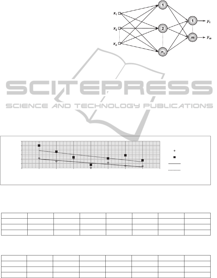
Figure 1 as a Fitting problem.

Figure 1: Neural Network (n=15 inputs, n

=12 hidden

neurons and m=8 outputs). Adapted from: (da Silva et al.,

2010).

5 PERFORMANCE

COMPARISON

The inferred data were compared with the observed

data using the ratio:









, where 



is the

population observed value and e 



the output value

of the inference where   1,…,167.

Figure 2: Linear tendency lines of means of all 167 samples from |Expected - Inferred| from each population.

Table 7: Maximum, Mean and Standard Deviation values for each population of calculated ratios









,

where





is the

observed value and e





the output value of the parameterized Bayesian inference where

  1,…,167.

Pop. 01 Pop. 02 Pop. 03 Pop. 04 Pop. 05 Pop. 06 Pop. 07

Max: 74.860000 70.501000 42.320600 38.680000 42.903000 50.782000 31.1506

Mean: 4.400000 2.940900 4.163577 0.084850 2.357600 0.996700 0.825800

SD: 13.847888 11.291766 6.209362 3.301484 7.728617 9.002339 5.766513

Table 8: Maximum, Mean and Standard Deviation values for each population of calculated ratios









, where





is the

observed value and e





the output value of the Neural Network where

  1,…,167.

Pop. 01 Pop. 02 Pop. 03 Pop. 04 Pop. 05 Pop. 06 Pop. 07

Max:

58.54958 45.93419 39.78041 9.130595 33.92973 36.03939 27.6264

Mean:

10.08046 7.251721 4.794875 1.405569 4.301284 5.668362 3.439153

SD:

10.83919 6.984214 5.140308 1.474641 4.97424 5.378425 4.046496

0,00

2,00

4,00

6,00

8,00

10,00

12,00

012345678

Mean of ratio

Population

Bayesian

ANN

Linear (Bayesian)

Linear (ANN)

BayesianversusNeuralNetworkAnalysisofAlgaeDataPopulation-ANewMethodtoPredictandAnalyseCauseand

Effect

487

For each population ratio column the maximum

value, the mean and the standard deviation were

extracted and are presented in Table 7 and Table 8.

The prediction performance of the Bayesian

inference shows a slightly better performance when

we analyze the linear tendency lines of the means of

ratios of each population (Figure 2), since it is lower

in the graph and nearer from 0, although, comparing

Table 7 and Table 8, the Standard Deviation in the

ANN approach is lower. Overall, performance of

both methods is similar.

6 CONCLUSIONS

In this work we provided a complete statistical

analysis method of a complex biological database,

including a method to mixture qualitative and

quantitative data, which can be used in several

inference models. Also, the regression model

associated to the compositional data analysis is a

powerful statistical tool to understand several

biological population data.

The Bayesian method may be improved and

other prior distributions for the parameters and/or

other error distributions in (2) can be used for a

better prediction performance. The ability to

evaluate the significance of each variable is an

important tool to maximize experiments resources

and understand biological processes. It is expected

with the improvement of the Bayesian inference

method, that less data could be necessary to train the

algorithm to acquire good regression parameters. It

is important to notice that previously knowledge of

the problem can be very useful to model the problem

and determine the best distributions for the

problems.

REFERENCES

Aitchison, J., 1982. The statistical analysis of

compositional data. Journal of the Royal Statistical

Society, pp. p. 139-177.

Aitchison, J., 1986. The statistical analysis of

compositional data. Chapman and Hall.

Aitchison, J. & Shen, S. M., 1980. Logistic-normal

distributions: Some properties and uses. Biometrika,

Issue 67, pp. 261-272.

da Silva, I. N., Spatti, D. H. & Flauzino, R. A., 2010.

Redes Neurais Artificiais para engenharia e ciências

aplicadas. I ed. São Paulo: ArtLiber.

Gelfand, A. E., Carlin, J. B., Stern, H. S. & Rubin, D. B.,

1995. Bayesian Data Analysis. Issue 85, pp. 398-409.

Gelfand, A. E. & Smith, A. F. M., 1990. Sampling based

approaches to calculating marginal densities. Journal

of the American Statistical Association, Issue 85, pp.

398-409.

Iyengar, M. & Dey, D. K., 1996. Bayesian Analysis of

Compositional Data. Department of Statistics,

University of Connecticut, Storrs, CT.

Iyengar, M. & Dey, D. K., 1998. Box-Cox transformations

in Bayesian analysis of compositional data.

Environmetrics, Issue 9, pp. 657-671.

López-Flores, R., Romaní, A. M. & Quintana, X. D.,

2011. Phytoplankton composition in shallow water

ecosystems: influence of environmental gradients and

nutrient availability, In 4

international Workshop on

Compositional Data Analysis.

Lynch, S. M., 2007. Introduction to Applied Bayesian

Statistics and Estimation for Social Scientists.

s.l.:Springer .

OpenBUGS, 2009. OpenBUGS, accessed 10 Feb 2013,

<http://www.openbugs.info/w.cgi/FrontPage>.

Rayens, W. S. & Srinivasan, C., 1991a. Box-Cox

transformations in the analysis of compositional data.

Journal of Chemometrics, Issue 5, pp. 227-239.

Rayens, W. S. & Srinivasan, C., 1991b. Estimation in

compositional data. Journal of Chemometrics, Issue 5,

pp. 361-374.

Roberts, G. O. & Smith, A. F. M., 1993. Bayesian

methods via the Gibbs sampler and related Markov

Chain Monte Carlo methods. Journal of the Royal

Statistical Society, 55(1), pp. 3-23.

The MathWorks, Inc., 1994-2013. Neural Network

Toolbox, accessed 20 Jan 2013, <http://

www.mathworks.com/products/neural-network/descri

ption2.html>.

Tjelmeland, H. & Lund, K. V., 2003. Bayesian modelling

of spatial compositional data, preprint n.1. Journal of

Applied Statistics, Issue 30, pp. 87-100.

Univesity of California - Irvine, 1999. COIL 1999

Competition Data, accessed 10 Jul 2013,

<http://kdd.ics.uci.edu/databases/coil/coil.data.html>.

IJCCI2013-InternationalJointConferenceonComputationalIntelligence

488