Enhancing Optimal Weight Tuning in H

Loop-shaping Control with
Particle Swarm Optimization
Philippe Feyel
1
, Gilles Duc
2
and Guillaume Sandou
2
1
SAGEM (SAFRAN Group), Optronics & Defense division, 100 Avenue de Paris, 91344 MassyCedex, France
2
SUPELEC Systems Sciences (E3S), Automatic Control Department, 3 rue Jolio-Curie, 91192 Gif-sur-Yvette, France
Keywords: Particle Swarm Optimization, H

Control, Loop-shaping.
Abstract: The H

loop-shaping controllers have proven their efficiency to solve problems based on complex industrial
specifications. However, the design is based on the tuning of weighting filters to reformulate all the
specifications, which is a time consuming task requiring know-how and expertise. This paper deals with the
use of Particle Swarm Optimization (PSO) algorithm for tuning the weighting filters. Whereas this topic has
already been investigated in lots of works especially using evolutionary algorithms, we propose here to
enhance the optimization process by working on the definition of a generic fitness function from a general
high-level specification, and by relaxing constraints on weights structure. The developed methodology is
tested using a real industrial example and leads to satisfactory results.
1 INTRODUCTION
H

synthesis is an efficient tool in robust control.
Among several design methodologies, the loop-
shaping procedure (McFarlane and Glover, 1992)
has strong advantages in the industrial framework. It
is based on the definition of weighting filters to
reformulate the desired specifications of the closed-
loop. An optimization step, based on the H

theory,
is then used to compute the final controller. The
main advantage of this design procedure is that the
weighting filter selection step allows the use of
linear transfer functions with decoupled intuition
and classical considerations on the open-loop gain
(bandwidth, low-frequency gain, etc). However,
choosing the “best” filters to capture as well as
possible complex specifications (mixing for instance
linear and nonlinear considerations) is difficult and
often time-consuming. Indeed, the classical
approach relies on an oriented “try and error”
procedure: the design problem is first simplified by
neglecting some nonlinear or disturbance
phenomena and/or some specifications. The
controller is then validated using time-domain
simulations of a full model. Several iterations are
thus generally needed in the development process.
Further, some expertise is often required to
reformulate specifications and to define well suited
weighting filters. This issue is worsened when the
final goal is not only to satisfy some specifications,
but also to optimize the closed-loop performance.
Since the emergence of H

theory, lots of works
have been done to optimize the weight selection
process. In (Lanzon, 2005) weighing functions are
set by a quasi-convex optimization problem.
Although effective, the main difficulty of such
approaches is related to the necessary open-loop
frequency specification framework used for the
optimization process. This is usually not
straightforward to obtain from a complex high-level
specification and the efficiency of the method often
relies on the expertise of the designer.
To avoid the frequency declination task, other
approaches based on stochastic optimization have
been considered. For instance in (Chipperfield,
Dakev, Fleming and Whidborne, 1996), weighing
functions of low order are selected with an
evolutionary algorithm. Based on stochastic
optimization, such works prove that complex criteria
can be considered in the Automatic control field
even if their gradients are not available, the only
requirement being the capability of evaluating the
fitness function.
The main improvements proposed in this paper
rely on:
 the definition of the fitness function. This is of
course a crucial point in the optimization procedure.
For that purpose, we propose a method to build a
120
Feyel P., Duc G. and Sandou G..
Enhancing Optimal Weight Tuning in H8 Loop-shaping Control with Particle Swarm Optimizations.
DOI: 10.5220/0004552801200127
In Proceedings of the 5th International Joint Conference on Computational Intelligence (ECTA-2013), pages 120-127
ISBN: 978-989-8565-77-8
Copyright
c
 2013 SCITEPRESS (Science and Technology Publications, Lda.)

generic cost function from a general high-level
specification.
 the structure of the weighting filters. Lot of
works consist in tuning all these filters in terms of
pole / zero / damping / natural frequency of their
transfer functions. Using this particular structure,
and looking only for positive parameters, the
corresponding filters are stable with stable inverses.
Although this is not mandatory for H

loop-shaping
synthesis, it is well known that stability of the
weighting filters is required in the standard
approach. However, for a given order, choosing the
best structure (poles / zeros / dampings) for the
weights to get the best solution to the design
problem is a difficult task. Unfortunately, the final
value of the fitness may clearly depend on this
structure. That is why we propose in this paper to
determine weighting functions without any
assumption on their structure; this can be done by
tuning directly the state-space representation. In that
case, we show that the optimization becomes fast
and efficient if the “tridiagonal form” for the state-
space matrix is used (McKelvey and Helmersson,
1996).
In section 2, the classical automatic control
formulation is briefly reminded and the advanced
tuning methodology called “H

loop-shaping” is
described. In section 3, we introduce the PSO
algorithm together with the variant used in this
work. In section 4, we enhance the optimal weights
tuning first with a generic method to construct the
fitness from a general specification, and then with
the tuning of unstructured weight filters. Section 5
shows the optimization procedure. Finally, we
illustrate our work with a concrete industrial
example in section 6, exhibiting much than
satisfactory results.
2 PLANT CONTROL USING H

LOOP-SHAPING SYNTHESIS
2.1 Controller Design Framework
Consider the generic closed-loop framework of
figure 1 (where s is the Laplace variable).
System
)(sG ),( sθK
Controller
+
+
+
-
r
u v
y
d
ε
Figure 1: Classical closed-loop framework.
A plant modelled by its transfer function
)(sG
has to be controlled to get the best performances.
The control input of the system is
v
and its output
is
y . The controller is denoted by the transfer
function
),(  sK . This controller depends of some
tuning parameters
 which have to be chosen to get
this optimal behaviour. Roughly speaking, the goal
of the closed loop is to assure that the output of the
system
y tracks the reference r and is not much
influenced by the disturbance
d
which should be
rejected.
For this closed-loop system, any performance
criterion (potentially complex (see example in
section 6) and based on the responses of y, u and/or
 to some particular test signals applied on inputs r
or d) is a function of the controller parameters.
2.2 H
∞
Loop-shaping Design
Very often, a Proportional Integral Derivative (PID)
controller is used to achieve satisfactory
performance (Åström and Hägglund, 1995).
However, when the system to control has Multi-
Inputs / Multi-Outputs or high and various
performances in terms of reference tracking, low
energy controls or disturbance rejection, this
classical approach may fail, and advanced control
methods such as H
∞
loop-shaping (McFarlane and
Glover, 1992) have to be used.
Considering the classical scheme of figure 1, the
basic problem of the H

loop-shaping method is the
following: for a given
0 
, find a controller K(s)
such that the H

-norm of the transfer function
between inputs r, d and outputs e, u is less than
 ,
that is :












)()(
)()(
sTsT
sTsT
udur
dr
(1)
where T
x

y
(s) denotes the closed-loop transfer
between input x and output y.
As an advantage, the minimal attainable value of
 can be a priori computed from the solution of 2
Riccati equations: let
 
CBA ,,
be a state-space
realization of
)(sG
; one obtains:
2/1
)(sup1








 YX
i
i
(2)
where
)(YX
i

denotes an eigenvalue of YX, and
EnhancingOptimalWeightTuninginH∞ Loop-shapingControlwithParticleSwarmOptimizations
121

0;0
0;0


YBBCYCYYAAY
XCCXBBXAXXA
TTT
TTT
(3)
Furthermore explicit formulae are available to
construct any controller achieving a value of

arbitrarily close to its minimal value:





)()(
)()(
:)(
txCtu
tBtxAx
sK
cc
cccc

(4)
with:


















1
2
2
2
IYXIZ
XBC
YCZB
CYCZXBBAA
T
c
T
c
TT
c
(5)
In order to tune the performance, a loop-shaping
procedure is included in the design, which can be
summarized as follows:
 At first, the open-loop gain is shaped by
choosing a precompensator
)(sW
i
and a
postcompensator
)(sW
o
, following the classical
rules of Automatic control;
 A controller
)(sK
p
is then computed by solving
(1) where
)(sG
is replaced by the loop-shaped
plant:
)()()()( sWsGsWsG
iop

(6)
 The final controller
)(sK
is obtained by merging
the pre- and postcompensators with the previous
controller:
)()()()( sWsKsWsK
opi

(7)
However the tuning of the post and precompensators
is a crucial point in the design procedure which
requires expertise to reformulate any high-level
specifications. The optimization of this tuning to
squeeze the reformulation step and to achieve better
performances is explained in the sequel.
3 THE PSO ALGORITHM
3.1 The Standard Version (Bratton and
Kennedy, 2007)
PSO is a metaheuristic optimization method inspired
by the social behavior of bird flocking or fish
schooling. Consider the following optimization
problem:
)(min xf
x 
(8)
P particles are moving in the search space. Each of
them has its own velocity, and is able to remember
where it has found its best performance. For a given
particle, we define a neighborhood as a subset of
particles it is able to communicate with. So at any
time each particle knows the best position achieved
so far by a particle of its own neighborhood. The
following notations are used:

k
p
x
(resp.
k
p
v
): position (resp. velocity) of particle
p at iteration;







k
p
k
p
k
p
xfxfb ,minarg
1

: best position found
by particle p until iteration k;





PxV
k
p
,...,2,1
: set of “friend neighbors” of
particle p at iteration k;


)(minarg
,
xfg
k
p
k
i
xVibx
k
p


: best position found by
the friend neighbours of particle p until iteration
k.
The particles move in the search space according to
the following transition rule:




11
21
1
.




k
p
k
p
k
p
k
p
k
p
k
p
k
p
k
p
k
p
vxx
xgcxbcvwv
(9)


is the element wise product;
 w is the inertia factor;
 c
1
and c
2
are accelerator coefficients, chosen as
random numbers generated by a uniform
distribution on some intervals



21
,0,,0 cc
respectively.
We use the following standard settings (Clerc,
2012) for this work:
 swarm size P = 10+
n
, where n is the
dimension of the optimization problem;

)2ln(5,0
21



cc
;



3)(dim 
k
p
xV
Several topologies exist for the design of subsets
)(
k
p
xV
. We use the social ring topologies (Bratton
and Kennedy, 2007) in which the neighborhood of a
particle is composed by the 3 other following ones;
this set does not depend on iteration k and is done at
the initialization. The inertia factor is defined using
the variant below.
IJCCI2013-InternationalJointConferenceonComputationalIntelligence
122

3.2 TVRandIW Custom Version
We use the Time Varying Random Inertia Weight
version of PSO defined in (Eberhart, 2001) in which
the inertia weight is a random number generated by
a uniform distribution on the interval
 1,5.0
. Note
that the mean value of the inertia factor is 0.75
which is the value used in (Clerc, 2012). By
randomizing w at each iteration, we create diversity
that makes this PSO version powerful for high
dimensional optimization problems.
4 ENHANCING OPTIMAL
WEIGHT TUNING
4.1 A Generic Fitness Function from a
General Specification
As said above a robust controller K(s) that satisfies
complex specifications of the form
11
yy 
,
22
yy 
, …,
mm
yy 
has to be found. Given a loop
structure (for instance figure 1) and assuming that all
specified signals can be evaluated e.g. by simulation,
the previous constrained problem can be
transformed into a non-constrained one by
introducing penalty functions, and reducing the
fitness function:





m
j
yy
cc
jjj
exfxfxf
1
'
)(),()(
(10)
Tuning these penalty functions, i.e. the coefficients
),'(
jj
y 
, is a crucial point in the optimization
process. To satisfy the specification, we have to
choose:
1,' 
jjj
yy
(11)
However, there is no sense to change a problem of
filter parameter tuning into a problem of
optimization parameter tuning. That is why we
propose in this work a systematic tuning rule, where
no parameter has to be chosen.
Consider the j
th
constraint. We note:
jjj
yy '
(12)
where
j

can be regarded as a security margin to
satisfy the specification
j
y
more easily. At the end
of the optimization, the order of magnitude of the
penalty function
 
'
jjj
yy
e

has to be close to
opt

and
j
y has to be at most
j
y
. Thus:
 
 
j
opt
jopt
yy
jjj
e




ln
'
(13)
Generally, it is efficient to choose
jjj
yy 3.01.0 
whereas for a loop-shaping
design problem, we expect the optimal  value to be
3
opt
.
4.2 General Filter Formalism for
Optimization
In this section, we want to relax any structural
constraint on weighting functions. Consider a
weighting filter, represented by its transfer function
given by (for a Single Input / Single Output system
(SISO)):
)(
)(
)(
1
0
1
0
sU
sY
ss
s
sW
W
W
n
j
j
j
n
n
i
i
i










(14)
This filter can also be represented by its state space
representation, given by:





)()()(
)()()(
:)(
tuDtxCty
tuBtxAtx
sW
WWW
WWW

(15)
where A is a
nn 
matrix and
W
x
is the state vector.
The following notation is used:







DC
BA
sW )(
(16)
As an advantage, it is well known that such a
representation is numerically better conditioned than
the transfer function. Further, it can be easily
extended to Multi-Input / Multi-Output (MIMO)
systems.
However the main drawback of such a
representation is the high number of parameters to
be determined. Indeed if n is the order of a SISO
filter W(s), the number of unknowns is (n+1)
2
in
comparison with 2n+1 for the transfer function
representation. Furthermore, the choice of the
matrices A, B, C, D is not unique.
A better approach consists in using the
tridiagonal matrix form for the state-space matrix. A
real tridiagonal matrix is a square real matrix having
non-zero elements only on the main, first super and
first sub diagonals:
EnhancingOptimalWeightTuninginH∞Loop-shapingControlwithParticleSwarmOptimizations
123




















nnn
nn
aa
a
a
aa
A
,1,1
,1
1,2
2,11,1
000
00
00
00
000



(17)
It is shown in (McKelvey and Helmersson, 1996)
that for any MIMO representation (A,B,C,D), there
exists a state-space representation (A’,B’,C’,D’) with
A’ in tridiagonal form such that (A,B,C,D) and
(A’,B’,C’,D’) are similar, that is they lead to the
same transfer function. Thus for the optimization
problem, we can assume the state-space matrix to be
tridiagonal without loss of generality, which reduces
the number of unknowns to 5n-1 in the SISO case,
that is the same order of magnitude than for the
transfer function representation.
For a n
u
n
y
MIMO filter W(s) of order n, the
unknown parameters can be collected into a vector x
defined by:















D
C
B
A
x
x
x
x
x
(18)
with:


































































u
u
nn
n
n
n
B
nn
nn
nn
A
b
b
b
b
b
b
x
a
a
a
a
a
a
x
,
,1
2,
2,1
1,
1,1
1,
1,2
,1
2,1
,
1,1
,







(19)
and:


































































uy
y
u
u
y
y
nn
n
n
n
D
nn
n
n
n
C
d
d
d
d
d
d
x
c
c
c
c
c
c
x
,
1,
,2
1,2
,1
1,1
,
1,
,2
1,2
,1
1,1
,








(20)
Note that we cannot say anything about the stability
of W(s) or W(s)
-1
because all the coefficients can
take any real values. This problem will be dealt with
in the sequel.
4.3 Search Space Transformation
If all parameters were strictly positive, a
transformation on the initial search space interval
could be used as follows:
],[],'['
],'['],[
'
10
10
)(log'
xxxxxx
xxxxxx
x
x
xx







(21)
This transformation enhances the sensitivity of the
algorithm because the smallest values of x have the
same weights than the highest due to the logarithm
function. Doing that it is possible to choose a large
search space interval for x.
However, because structural constraints on
weights have been previously relaxed, unknowns
can be positive or negative. With the same idea, a
change of variable can be done by adapting the
previous logarithmic transformation with the
following functions:
2
1010
)(sh
1log)(ash
10
2
1010
xx
x
xxx










(22)
Thus, the following transformation on the initial
search space interval can be computed:
],[],'['
],'['],[
)'(sh
M
1
)(ash'
10
10
xxxxxx
xxxxxx
xx
Mxx








(23)
The function ash
10
(x) is close to log
10
(x) for high
values of
x
; but these functions are quite different
when
x
is close to 0. To make the smallest values
of
x
having the same weights than the highest ones
a scaling factor M >> 1 has to be used.
5 OPTIMIZATION PROCEDURE
The optimization consists in tuning the weighting
functions W
i
(s) and W
o
(s) defined as follows:














ii
ii
i
oo
oo
o
DC
BA
sW
DC
BA
sW )(,)(
(24)
IJCCI2013-InternationalJointConferenceonComputationalIntelligence
124

The decision variables are the corresponding
coefficients of their tridiagonal state-space
representation. The optimization can be done using
PSO.
As for a classical Automatic control design, we
constraint the weights filters to be stable and their
inverses too. For that purpose, the first task of the
optimization process consists in insuring these
stability constraints, as explained below.
Denote
A
 the eigenvalues of A. Assuming that
D
-1
exists, the state space matrix A of the inverse of
the system (A,B,C,D) is:
CBDAA
1

(25)
At the iteration k after moving the swarm according
to (9), do for each particle
k
p
x
:
 Build

oooo
DCBA ,,,
and

iiii
DCBA ,,,
from
k
p
x
;
 Evaluate
oooo
o
CDBAA
1
 and
iiii
i
CDBAA
1
 ;
 Evaluate:
))(realmax()),(realmax(
))(realmax()),(realmax(
i
A
i
A
o
A
o
A
i
A
i
A
o
A
o
A



0or0or0or0If 
i
A
o
A
i
A
o
A
,
evaluate:
i
A
o
A
i
A
o
A
eeeexf
k
p




.10
10
.10.10
)(
 Else:
 build W
i
(s) and W
o
(s) according to (16);
 build the loop-shape according to (6);
 compute K
p
(s) satisfying criterion (1);
 evaluate ;
 build the controller K(s) according to (7);
 evaluate f
c
according to (10);
 evaluate
c
k
p
f
xf


1
)(
 Find
 
)(),(minarg
1 k
p
k
p
k
p
xfxfb


;
Before moving the swarm at next iteration, the best
neighbor of each particle has to be identified:
 Finally find

)(minarg
,
xfg
k
p
k
i
xVibx
k
p


;
and go to next step.
The fitness function has been adapted to take into
account the stabilization task of the weights and
their inverses, which consists in rendering the real
part of the eigenvalues strictly negative using hard
penalty functions. When the weights and their
inverses just become stable, their poles are close to
the imaginary axis such that the  values obtained
with the corresponding controllers are high and so
 
1

c
fγ
is negative but close to 0. Thus, there is
continuity in the fitness function between the
stabilization task where the fitness is positive close
to 0 and the optimization task with an existing
controller where the fitness is negative close to 0.
6 INDUSTRIAL EXAMPLE:
INERTIAL LINE OF SIGHT
STABILIZATION
6.1 Problem Statement
To illustrate that work we choose a two axis Line Of
Sight (LOS) stabilization platform. The goal is to
maintain the LOS orientation fixed in an inertial
space, by rotating the gimbals via a gyrometric
feedback loop with inertial measures of the gimbals
motion, in spite of environmental conditions. For
further details in gyrostabilized viewfinder, refer to
(Masten, 2008) and (Hilkert, 2008) which give an
exhaustive description of the different possible
architectures. One considers the azimuth axis as a
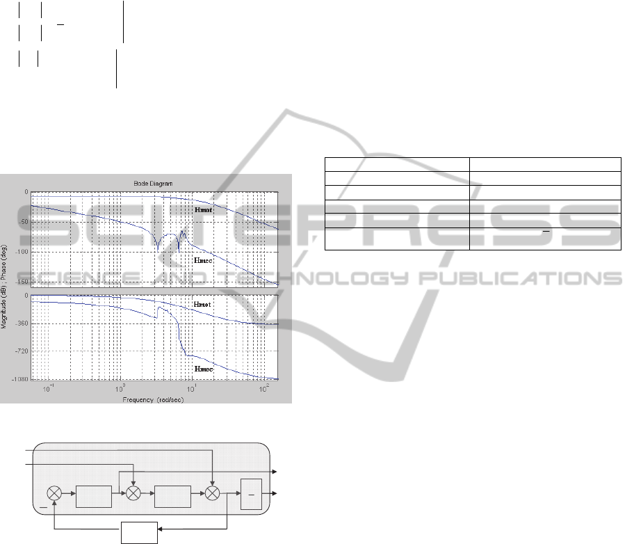
SIMO transfer function (figure 2) whose input is the
motor voltage u(t) and outputs are the inertial
velocity
 (t) measured by a gyrometer and the
motor current i(t):
)()(
1
)(
)(
)(
susH
sH
si
sΩ
mot
mec

















(26)
The inertial LOS stabilization problem consists in
rejecting two types of disturbances:
 The first one is the friction torque

f
(t) induced
by the rotational movements of the vehicle
supporting the platform. In this work, friction
torque is modeled by a Coulomb step:
0)(
0
 t,ΓtΓ
f
(27)
 The second one is the structural flexure
disturbance induced by the vehicle vibrations
that can make the LOS be chattering. In this
work, this disturbance is modeled by the
following noisy sine:
  0,sin)()(
00
 ttωVtvtΓ
v
(28)
EnhancingOptimalWeightTuninginH∞Loop-shapingControlwithParticleSwarmOptimizations
125

The control scheme is depicted in figure 3. Denoting
the angular performance
 (t), the goal is to find a
robust controller K(s) that guarantees the following
specifications:
)(toresponsein
0,)(
)(toresponsein
,)(
0,)(
max
max
max
tΓ
σσ
titi
tΓ
ttθtθ
tθtθ
v
θ
f
f




(29)
where 

is the standard deviation of  (t). Due to
confidentiality reasons, all the frequencies,
magnitudes of disturbances and specifications have
been normalized.
Figure 2: SIMO plot responses.
H
mot
(s) H
mec
(s)
K(s)

(t)
s
1

(t)
i(t)

f
(t)

v
(t)
u(t)
Figure 3: LOS control scheme.
6.2 Controller Synthesis
A SISO controller is designed with the H

loop-
shaping procedure. Thus an unstructured weight
W(s) is chosen with order 12.
Because PSO is a stochastic algorithm, it has to
be run several times to get a statistical validation and
evaluation of its performance (10 times in our case,
each of them involving 500 iterations). Note that an
optimization using 500 iterations needs 2 hours on a
CPU E7200 2.53 GHZ which is quite reasonable for
an off-line design of controllers. The best results
found are presented in table 1. As we can see, the
specification is entire satisfied. Note that with the
classical approach, an expert might find a controller
which achieves similar performances, but the
oriented ‘try and error’ approach based on
specifications reformulations would require several
days in comparison to the 20 hours of our
optimization (2 hours for each run).
Further, it exists some efficient methods to
compute low-order H

controllers (Apkarian, 2002),
(Gumussoy, 2008), but to our knowledge none of
them avoid the reformulation step and the definition
of well suited filters.
Table 1: Optimization results.
Specification Optimizing W(s)

o
p
t
3.9
max(|

(t)|) 0.32

max
max(|i(t)|) 0.9i
max


1.1

max
max(|  (t)| / t>t
f
)
θ
7 CONCLUSIONS
In this paper, we proposed to control a plant using
the H

loop-shaping method by tuning directly the
weighting filters according to the required
specifications using a PSO algorithm. Several
advantages have to be noticed. First, the use of an
optimization procedure provides a controller which
is supposed to be better than a controller tuned “by
hand”. Then the try and error classical procedure has
no more to be done, leading to less time-consuming
design process. Finally, the use of generic tuning
strategies of penalty functions leads to a zero
parameter methodology.
The proposed methodology has been tested on an
industrial problem. Our work showed the impact of
structural considerations on weighting filters: no
structural assumption is needed for the filter tuning
problem, allowing more degrees of freedom in the
design. Our future works consist in merging this
weighting filter selection problem with the problem
of finding a fixed order controller by the same way.
Note that all considerations of this work can also be
extended to other design methods such as the H

standard synthesis problem for example.
REFERENCES
Apkarian, P., Noll , D., 2002. Nonsmooth H

synthesis,.
In
Journal of class files, vol.1, n°11, November 2002.
IJCCI2013-InternationalJointConferenceonComputationalIntelligence
126

Åström, K., Hägglund, T. 1995. PID controllers: Theory,
Design, and tuning,
ISA edition
Bratton, B., Kennedy, J., 2007. Defining a standard for
particle swarm optimization. In IEEE Swarm. Intel.
Symp., April 2007, pp 120-127
.
Chipperfield, A. J., Dakev, N. V., Fleming, P. J.,
Whidborne J. F, 1996. Multiobjective robust control
using evolutionary algorithm. In
IEEE Inter. Conf. on
Indus. Techno., Dec 1993, pp. 269-273
.
Clerc M., 2012. Standard Particle Swarm Optimization. In
http://clerc.maurice.free.fr/pso, 2012
Eberhart, R.C., 2001. Tracking and optimizing dynamic
systems with particle swarms. In
IEEE. Evol. Comput.,
vol.1, 2001, pp 94-100
.
Gumussoy, S., Overton, M.L., 2008. Fixed-order H

controller design via HIFOO, a specialized nonsmooth
package. In
2008 America Control Conference Westin
Seattle Hotel,
Seatle, Washington, USA, June 11-13
2008.
Hilkert, J.M, 2008. Inertially Stabilized Platforms
Technology. In
IEEE Control Systems Magazine,
28(1):26-46.
Lanzon, A., 2005. Weight optimization in H

loop-
shaping,. In
Automatica, vol.41, 2005, pp. 1201-1208.
Masten, M. K., 2008. Inertially Stabilized Platforms for
Optical Imaging Systems. In IEEE Control Systems
Magazine,
28(1):47-64.
McFarlane, D., Glover, K., 1992. A loop-shaping design
procedure using H

synthesis. In IEEE Trans. Autom
control,
vol. 37, No 6, June 1992, pp. 759-769.
McKelvey, T., Helmersson, A., 1996. State-space
parameterizations of multivariable linear systems
using tridiagonal matrix forms. In
35th IEEE. Decision
and control conf.,
vol.4, Dec 1996, pp 3654-3659.
EnhancingOptimalWeightTuninginH∞Loop-shapingControlwithParticleSwarmOptimizations
127