
The L-Co-R Co-evolutionary Algorithm
A Comparative Analysis in Medium-term Time-series Forecasting Problems
E. Parras-Gutierrez
1
, V. M. Rivas
1
and J. J. Merelo
2
1
Department of Computer Sciences, University of Jaen, Campus Las Lagunillas s/n, 23071, Jaen, Spain
2
Department of Computers, Architecture and Technology, University of Granada,
C/ Periodista Daniel Saucedo s/n, 18071, Granada, Spain
Keywords:
Time Series Forecasting, Co-evolutionary Algorithms, Neural Networks, Significant Lags.
Abstract:
This paper presents an experimental study in which the effectiveness of the L-Co-R method is tested. L-
Co-R is a co-evolutionary algorithm to time series forecasting that evolves, on one hand, RBFNs building
an appropriate architecture of net, and on the other hand, sets of time lags that represents the time series in
order to perform the forecasting using, at the same time, its own forecasted values. This coevolutive approach
makes possible to divide the main problem into two subproblems where every individual of one population
cooperates with the individuals of the other. The goal of this work is to analyze the results obtained by L-Co-R
comparing with other methods from the time series forecasting field. For that, 20 time series and 5 different
methods found in the literature have been selected, and 3 distinct quality measures have been used to show the
results. Finally, a statistical study confirms the good results of L-Co-R in most cases.
1 INTRODUCTION
Formally defined, a time series is a set of observed
values from a variable along time in regular periods
(for instance, every day, every month or every year)
(Pe
˜
na, 2005). Accordingly, the work of forecasting in
a time series can be defined as the task of predicting
successive values of the variable in time spaced based
on past and present observations.
For many decades, different approaches have been
used for to modelling and forecasting time series.
These techniques can be classified into three different
areas: descriptive traditional technologies, linear and
nonlinear modern models, and soft computing tech-
niques. From all developed method, ARIMA, pro-
posed by Box and Jenkins (Box and Jenkins, 1976), is
possibly the most widely known and used. Neverthe-
less, it yields simplistic linear models, being unable
to find subtle patterns in the time series data.
New methods based on artificial neural networks,
such as the one used in this paper, on the other hand,
can generate more complex models that are able to
grasp those subtle variations.
The L-Co-R method (Parras-Gutierrez et al.,
2012), developed inside the field of ANNs, makes
jointly use of Radial Basis Function Networks
(RBFNs) and EAs to automatically forecast any given
time series. Moreover, L-Co-R designs adequate neu-
ral networks and selects the time lags that will be
used in the prediction, in a coevolutive (Castillo et al.,
2003) approach that allows to separate the main prob-
lem in two dependent subproblems. The algorithm
evolves two subpopulations based on a cooperative
scheme in which every individual of a subpopulation
collaborates with individuals from the other subpopu-
lation in order to obtain good solutions.
While previously work (Parras-Gutierrez et al.,
2012) was focused on 1-step ahead prediction, the
main goal of this one is to analyze the effectiveness
of the L-Co-R method in the medium-term horizon,
using the own previously predicted values to perform
next predictions. For this reason, L-Co-R has been
tested over 20 databases, taken from real world, or
used in well-known research publications and time
series competition. As section 4 shows, the method
has been compared against 5 time series forecasting
methods.
The rest of the paper is organized as follows: sec-
tion 2 introduces some preliminary topics related to
this research; section 3 describes the method L-Co-R;
section 4 presents the experimentation and the statis-
tical study carried out, while section 5 presents some
conclusions of the work.
144
Parras-Gutierrez E., M. Rivas V. and Merelo J..
The L-Co-R Co-evolutionary Algorithm - A Comparative Analysis in Medium-term Time-series Forecasting Problems.
DOI: 10.5220/0004555101440151
In Proceedings of the 5th International Joint Conference on Computational Intelligence (ECTA-2013), pages 144-151
ISBN: 978-989-8565-77-8
Copyright
c
2013 SCITEPRESS (Science and Technology Publications, Lda.)

2 PRELIMINARIES
Approaches proposed in time series forecasting can
be mainly grouped as linear and nonlinear models.
Methods like exponential smoothing methods (Win-
ters, 1960), simple exponential smoothing, Holt’s lin-
ear methods, some variations of the Holt-Winter’s
methods, State space models (Snyder, 1985), and
ARIMA models (Box and Jenkins, 1976), have stand
out from linear methods, used chiefly for modelling
time series. Nonlinear models arose because linear
models were insufficient in many real applications;
between nonlinear methods it can be found regime-
switching models, which comprise the wide variety
of existing threshold autoregressive models (Tong,
1978). Nevertheless, soft computing approaches were
developed in order to save disadvantages of nonlinear
models like the lack of robustness in complex model
and the difficulty to use (Clements et al., 2004).
ANNs have also been successfully applied (Jain
and Kumar, 2007) and recognized as an important tool
for time-series forecasting. Within ANNs, the utiliza-
tion of RBFs as activation functions were considered
by works as (Broomhead and Lowe, 1988) and (Rivas
et al., 2004), while Harpham and Dawson (Harpham
and Dawson, 2006) or Du (Du and Zhang, 2008) fo-
cused on RBFNs for time series forecasting.
On the other hand, an issue that must be taken
into account when working with time series is the cor-
rect choice of the time lags for representing the series.
Takens’ theorem (Takens, 1980) establishes that if d,
a d-dimensional space where d is the minimum di-
mension capable of representing such a relationship,
is sufficiently large is possible to build a state space
using the correct time lags and if this space is cor-
rectly rebuilt also guarantees that the dynamics of this
space is topologically identical to the dynamics of the
real systems state space.
Many methods are based in Takens’ theorem (like
(Lukoseviciute and Ragulskis, 2010)) but, in gen-
eral, the approaches found in the literature consider
the lags selection as a pre or post-processing or as
a part of the learning process (Ara
´
ujo, 2010),(Maus
and Sprott, 2011). In the L-Co-R method the selec-
tion of the time lags is jointly faced along with the
design process, thus it employs co-evolution to simul-
taneously solve these problems.
Cooperative co-evolution (Potter and De Jong,
1994) has also been used in order to train ANNs
to design neural network ensembles (Garc
´
ıa-Pedrajas
et al., 2005) and RBFNs (Li et al., 2008). But in addi-
tion, cooperative co-evolution is utilized in time series
forecasting in works as the one by Xin (Ma and Wu,
2010).
3 DESCRIPTION OF THE
METHOD
This section describes L-Co-R (Parras-Gutierrez
et al., 2012), a co-evolutionary algorithm developed
to minimize the error obtained for automatically time
series forecasting. The algorithm works building at
the same time RBFNs and sets of lags that will be
used to predict future values. For this task, L-Co-R
is able to simultaneously evolve two populations of
different individual species, in which any member of
each population can cooperate with individuals from
the other one in order to generate good solutions, that
is, each individual represents itself a possible solution
to the subproblem. Therefore, the algorithm is com-
posed of the following two populations:
• Population of RBFNs: it consists of a set of
RBFNs which evolves to design a suitable ar-
chitecture of the network. This population em-
ploys real codification so every individual repre-
sent a set of neurons (RBFs) that composes the
net. Each neuron of the net is defined by a center
(a vector with the same dimension as the inputs)
and a radius. The exact dimension of the input
space is given by an individual of the population
of lags (the one chosen to evaluate the net). Dur-
ing the evolutionary process neurons can grow or
decrease since the number of neurons is variable,
and centers and radius can also be modified by
means of muatation.
• Population of lags: it is composed of sets of lags
evolves to forecast future values of the time series.
The population uses a binary codification scheme
thus each gene indicates if that specific lag in the
time series will be utilized in the forecasting pro-
cess. The length of the chromosome is set at the
beginning corresponding with the specific param-
eter, so that it cannot vary its size during the exe-
cution of the algorithm.
As the fundamental objective, L-Co-R forecasts
any time series for any horizon and builds appropriate
RBFNs designed with suitable sets of lags, reducing
any hand made preprocessing step. Figure 1 describes
the general scheme of the algorithm L-Co-R.
L-Co-R performs a process to automatically re-
move the trend of the times series to work with, if
necessary. This procedure is divided into two main
phases: preprocessing, which takes places at the be-
ginning of the algorithm, and post-processing, at the
end of co-evolutionary process. Basically, the algo-
rithm checks if the time series includes trend and, in
affirmative case, the trend is removed.
TheL-Co-RCo-evolutionaryAlgorithm-AComparativeAnalysisinMedium-termTime-seriesForecastingProblems
145

Trend preprocessing
t = 0;
initialize P lags(t);
initialize P RBFNs(t);
evaluate individuals in P lags(t);
evaluate individuals in P RBFNs(t);
while termination condition not satisfied do
begin
t = t+1;
/* Evolve population of lags */
for i=0 to max gen lags do
begin
set threshold;
select P lags’(t) from P lags(t);
apply genetic operators in P lags’(t);
/* Evaluate P lags’(t) */
choose collaborators from P RBFNs(t);
evaluate individuals in P lags’(t);
replace individuals P lags(t) with P lags’(t);
if threshold < 0
begin
diverge P lags(t);
end
end
/* Evolve population of RBFNs */
for i=0 to max gen RBFNs do
begin
select P RBFNs’(t) from P RBFNs(t);
apply genetic operators in P RBFNs’(t);
/* Evaluate P RBFNs’(t) */
choose collaborators from P lags(t);
evaluate individuals in P RBFNs’(t);
replace individuals with P RBFNs’(t);
end
end
train models and select the best one
forecast test values with the final model
Trend postprocessing
Figure 1: General scheme of method L-Co-R.
The performance of L-Co-R starts with the cre-
ation of the two initial populations, randomly gener-
ated for the first generation; then, each individual of
the populations is evaluated. The L-Co-R algorithm
uses a sequential scheme in which only one popu-
lation is active, so the two population take turns in
evolving. Firstly, the evolutionary process of the pop-
ulation of lags occurs: the individuals which will be-
long to the subpopulation are selected; following the
CHC scheme (Eshelman, 1991), genetic operators are
applied; the collaborator for every individual is cho-
sen from the population of RBFNs; and the individu-
als are evaluated again and assigned the result as fit-
ness. After that, the best individuals from the sub-
population will replace the worst individuals of the
population. During the evolution, the population of
lags checks that al least one gene of the chromosome
must be set to one because necessarily the net needs
one input to obtained the forecasted value.
In the second place, the population of RBFNs
starts the evolutionary process. For the first gener-
ation, every net in the population has a number of
neurons randomly chosen which may not exceed a
maximum number previously fixed. As in population
of lags, the individuals for the subpopulation are se-
lected, the genetic operators are applied, every indi-
vidual chooses the collaborator from the population
of lags, and then, the individuals are evaluated and
the result is assigned as fitness. Fitness function is
defined by the inverse of the root mean squared error
At the end of the co-evolutionary process, two mod-
els formed by a set of lags (from the first population)
and a neural network (from the second population) are
obtained. On the one hand, a model is composed of
the best set of lags and its best collaborator, and on
the other hand, the other model is composed of the
best net found and its best collaborator. Then, the two
models are trained again and the final model chosen is
the one that obtains the best fitness. This final model
obtains the future values of the time series used for
the prediction, and then, forecasted data will be used
to find next values.
The collaboration scheme used in L-Co-R is the
best collaboration scheme (Potter and De Jong, 1994).
Thus, every individual in any population chooses the
best collaborator from the other population. Only at
the beginning of the co-evolutionary process, the col-
laborator is selected randomly because the population
has not been evaluated yet.
The method has a set of specific operators spe-
cially developed to work with individuals from every
population. The operators used by L-Co-R are the fol-
lowings:
• Population of RBFNs: tournament selection, x fix
crossover, four operators to mutate randomly cho-
sen (C random, R random, Adder, and Deleter)
and replacement of the worst individuals by the
best ones of the subpopulation.
• Population of lags: elitist selection, HUX
crossover operator, replacement of the worst in-
dividuals, and diverge (the population is restarted
when it is blocked).
IJCCI2013-InternationalJointConferenceonComputationalIntelligence
146

4 EXPERIMENTATION AND
STATISTICAL STUDY
The main goal of the experiments is to study the be-
havior of the algorithm L-Co-R comparing with other
5 methods found in the literature and for 3 different
quality measures.
4.1 Experimental Methodology
As in (Parras-Gutierrez et al., 2012), the experimen-
tation has been carried out using 20 data bases, most
of then taken from the INE
1
. The data represent ob-
servations from different activities and have differ-
ent nature, size, and characteristics. The data bases
have been labeled as: Airline, WmFrancfort, Wm-
London, WmMadrid, WmMilan, WmNewYork, Wm-
Tokyo, Deceases, SpaMovSpec, Exchange, Gasoline,
MortCanc, MortMade, Books, FreeHouPrize, Prison-
ers, TurIn, TurOut, TUrban, and HouseFin. The num-
ber of samples in every database is between 43 (for
MortCanc) and 618 (for Gasoline, a database used in
the NN3 competition).
To compare the effectiveness of L-Co-R, 5 ad-
ditional methods have been used, all of them found
within the field of time series forecasting: Exponen-
tial smoothing method (ETS), Croston, Theta, Ran-
dom Walk (RW), and ARIMA (Hyndman and Khan-
dakar, 2008).
In order to test and compare the generalization ca-
pabilities of every method, databases have been split
into training and test sets. Training sets have been
given the first 75% of the data, while test sets are com-
posed by the remaining 25% samples.
An open question when dealing with time series is
the measure to be used in order to calculate the accu-
racy of the obtained predictions. Mean Absolute Per-
centage Error (MAPE) (Bowerman et al., 2004) was
intensively used until many other measures as Geo-
metric Mean Relative Absolute Error, Median Rel-
ative Absolute Error, Symmetric Median and Me-
dian Absolute Percentage Error (MdAPE), or Sym-
metric Mean Absolute Percentage Error were pro-
posed (Makridakis and Hibon, 2000). However, a
disadvantage was found in these measures, they were
not generally applicable and can be infinite, unde-
fined or can produce misleading results, as Hyndman
and Koehler explained in their work (Hyndman and
Koehler, 2006). Thus, they proposed Mean Absolute
Scaled Error (MASE) that is less sensitive to outliers,
less variable on small samples, and more easily inter-
preted.
1
National Statistics Institute (http://www.ine.es/)
In this work, the measures used are MAPE (i.e.,
mean(| p
t
|)), MASE (defined as mean(| q
t
|)), and
MdAPE (as median(| p
t
|) ), taking into account that
Y
t
is the observation at time t = 1, ...,n; F
t
is the fore-
cast of Y
t
; e
t
is the forecast error (i.e. e
t
= Y
t
− F
t
);
p
t
= 100e
t
/Y
t
is the percentage error, and q
t
is deter-
mined as:
q
t
=
e
t
1
n − 1
n
∑
i=2
| Y
i
−Y
i−1
|
Due to its stochastic nature, the results yielded by
L-Co-R have been calculated as the average errors
over 30 executions with every time series. For each
execution, the following parameters are used in the
L-Co-R algorithm: lags population size=50, lags pop-
ulation generations=5, lags chromosome size=10%,
RBFNs population size=50, RBFNs population gen-
erations=10, validation rate=0.25, maximum num-
ber of neurons of first generation=0.05, tournament
size=3, replacement rate=0.5, crossover rate=0.8, mu-
tation rate=0.2, and total number of generations=20.
Tables 1, 2, and 3 show the results of the L-Co-
R and the utilized methods to compare (ETS, Cros-
ton, Theta, RW, and ARIMA), for measures MAPE,
MASE, and MdAPE, respectively (best results are
emphasized with the character *). As mentioned be-
fore, every result indicated in the tables represent the
average of 30 executions for each time series. With
respect to MAPE, the L-Co-R algorithm obtains the
best results in 15 of 20 time series used, as can be
seen in table 1. Regarding MASE, L-Co-R stands out
yielding the best results for 5 time series; ETS, Cros-
ton and Theta for 3 time series; RW only for 2; and
ARIMA for 4 time series; as can be observed in ta-
ble 2. Concerning MdAPE, L-Co-R acquires better
results than the other methods in 12 of 20 time series,
as table 3 shows. Thus, the L-Co-R algorithm is able
to achieve a more accurate forecast in the most time
series for any of the quality measures considered.
4.2 Analysis of the Results
To analyze in more detail the results and check
whether the observed differences are significant, two
main steps are performed: firstly, identifying whether
exist differences in general between the methods used
in the comparison; and secondly, determining if the
best method is significant better than the rest of the
methods. To do this, first of all it has to be decided if
is possible to use parametric o non-parametric statisti-
cal techniques. An adequate use of parametric statis-
tical techniques reaching three necessary conditions:
independency, normality and homoscedasticity (She-
skin, 2004).
TheL-Co-RCo-evolutionaryAlgorithm-AComparativeAnalysisinMedium-termTime-seriesForecastingProblems
147

Table 1: Results of the methods L-Co-R, ETS, Croston, Theta, RW, and ARIMA, with respect to MAPE. Best result per
database is marked with character *.
Time series L-Co-R ETS Croston Theta RW ARIMA
Airline 30.380 * 274.770 72.606 141.452 137.986 53.636
WmFrancfort 16.423 17.393 40.544 22.745 25.169 12.136 *
WmLondon 2.860 * 5.383 27.682 10.136 13.397 5.212
WmMadrid 20.101 27.035 44.285 25.505 27.034 12.930 *
WmMilan 30.529 * 34.858 49.750 34.078 34.823 34.823
WmNewYork 8.259 7.182 * 30.297 14.669 18.073 7.536
WmTokyo 4.764 * 12.807 20.556 10.575 12.591 12.591
Deceases 5.981 * 8.002 7.472 7.264 8.040 8.040
SpaMovSpec 53.788 * 217.978 78.648 70.500 78.935 88.197
Exchange 43.044 46.025 31.121 * 39.138 33.631 45.254
Gasoline 1.654 * 7.986 9.587 6.701 7.974 9.359
MortCanc 1.137 * 12.979 32.489 5.889 6.256 5.440
MortMade 3.931 * 13.526 46.362 40.272 12.800 31.000
Books 13.787 * 23.588 23.122 22.360 22.640 23.476
FreeHouPrize 3.424 * 8.540 29.271 5.215 9.220 10.227
Prisoners 8.392 3.103 * 14.220 6.888 9.474 3.150
TurIn 1.357 * 7.074 11.234 7.084 7.110 6.377
TurOut 8.133 * 13.261 12.159 15.238 13.226 9.634
TUrban 2.734 * 11.957 9.067 8.949 10.116 9.291
HouseFin 16.452 * 22.296 21.548 19.947 22.887 19.555
Table 2: Results of the methods L-Co-R, ETS, Croston, Theta, RW, and ARIMA, with respect to MASE. Best result per
database is marked with character *.
TS L-Co-R ETS Croston Theta RW ARIMA
Airline 1.913 12.707 2.738 5.853 5.664 1.441 *
WmFrancfort 3.578 * 3.608 7.984 4.673 5.159 7.988
WmLondon 1.648 1.603 * 8.410 3.099 4.119 3.484
WmMadrid 4.442 * 5.686 9.126 5.362 5.685 8.625
WmMilan 5.967 * 6.684 9.263 6.534 6.678 19.327
WmNewYork 2.667 1.837 * 7.982 3.942 4.879 6.228
WmTokyo 2.791 2.443 3.935 2.129 2.402 1.628 *
Deceases 1.059 1.059 0.952 * 0.955 1.064 1.144
SpaMovSpec 1.027 2.027 1.009 * 1.023 1.010 1.933
Exchange 41.181 44.039 30.448 * 37.807 32.825 70.734
Gasoline 1.198 * 1.543 1.864 1.274 1.541 1.698
MortCanc 0.646 1.618 4.098 0.725 0.796 0.277 *
MortMade 1.314 1.303 * 4.500 3.869 1.315 1.712
Books 0.762 0.965 0.936 0.894 0.759 * 1.147
FreeHouPrize 3.339 * 5.642 19.468 3.487 6.183 6.805
Prisoners 14.482 5.485 23.979 11.934 16.305 4.031 *
TurIn 1.903 1.902 3.151 1.824 * 1.916 1.950
TurOut 2.005 2.000 2.088 2.239 1.996 * 2.241
TUrban 0.886 0.978 0.772 0.744 * 0.887 0.897
HouseFin 1.319 1.283 1.234 1.095 * 1.322 1.502
Owing to the former conditions are not fulfilled,
the Friedman and Iman-Davenport non-parametric
tests have been used. Tables 4 and 5 shows the results
for MAPE, MASE and MdAPE, for these tests. From
left to right, tables show the Friedman and Iman-
Davenport values (χ
2
and F
F
, respectively), the cor-
responding critical values for each distribution by us-
ing a level of significance α = 0.05, and the p-value
obtained for the measures utilized.
As can be observed, the critical values of Fried-
IJCCI2013-InternationalJointConferenceonComputationalIntelligence
148
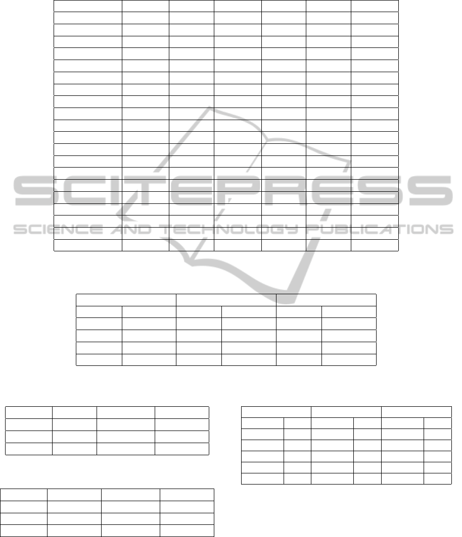
Table 3: Results of the methods L-Co-R, ETS, Croston, Theta, RW, and ARIMA, with respect to MdAPE. Best result per
database is marked with character *.
Time series L-Co-R ETS Croston Theta RW ARIMA
Airline 15.057 * 233.934 54.657 119.754 118.090 15.212
WmFrancfort 14.610 14.603 39.259 19.960 22.750 11.026 *
WmLondon 3.498 * 5.430 30.550 10.474 15.722 5.099
WmMadrid 22.718 28.116 45.817 26.787 28.116 11.446 *
WmMilan 30.476 * 34.685 50.040 33.872 34.643 34.643
WmNewYork 9.114 4.598 * 35.253 16.505 23.137 5.712
WmTokyo 5.517 * 9.864 18.782 9.075 9.556 9.556
Deceases 4.267 * 5.464 6.121 4.440 5.458 5.458
SpaMovSpec 17.669 * 107.283 51.653 53.104 51.568 54.033
Exchange 44.368 46.597 34.121 * 38.832 36.521 45.961
Gasoline 1.792 * 7.587 9.045 6.429 7.563 8.923
MortCanc 11.25 9.694 30.568 4.047 * 5.339 5.116
MortMade 3.459 * 12.111 45.704 41.989 15.629 28.374
Books 4.868 * 18.111 17.230 16.566 11.567 18.093
FreeHouPrize 1.803 * 5.222 29.683 5.201 9.748 6.572
Prisoners 6.766 1.512 * 12.651 5.287 7.817 1.621
TurIn 2.945 * 6.627 11.696 4.779 6.669 4.605
TurOut 5.289 * 11.331 11.518 10.873 11.392 7.689
TUrban 5.290 8.262 6.822 4.922 * 8.900 6.374
HouseFin 18.286 22.623 21.279 18.845 23.684 17.297 *
Table 7: Adjusted p values of Holm’s procedure between the control algorithm (L-Co-R) and the other methods for MAPE,
MASE, and MdAPE. Values lower than alpha = 0.05 indicate significant differences between L-Co-R and the corresponding
algorithm.
MAPE MASE MdAPE
Croston 2.433E-08 ARIMA 1.138E-03 Croston 2.432E-08
ETS 3.346E-06 Croston 1.528E-03 ETS 1.692E-04
RW 9.120E-06 ETS 1.083E-01 RW 2.002E-04
ARIMA 4.636E-03 RW 1.179E-01 Theta 6.298E-02
Theta 5.287E-03 Theta 7.673E-01 ARIMA 6.920E-02
Table 4: Results of the Friedman, showing signficant differ-
ences as p −values < 0.05.
Measure F. Value Value in χ
2
p value
MAPE 39.364 5 2.101E-10
MASE 18.893 5 2.012E-03
MdAPE 38.350 5 3.209E-07
Table 5: Results of the Iman-Davenport test, showing sign-
ficant differences as p − values < 0.05.
Measure I-D. Value Value in F
F
p value
MAPE 12.283 5 and 95 3.416E-09
MASE 4.426 5 and 95 1.146E-03
MdAPE 11.819 5 and 95 6.717E-09
man and Iman-Davenport are smaller than the statis-
tic, it means that there are significant differences
among the methods in all cases. In addition, Fried-
man provides a ranking of the algorithms, so that the
method with a lowest result is taken as the control al-
Table 6: Friedman’s test ranking. Control algorithms are
located in first row.
MAPE MASE MdAPE
L-Co-R 1.50 L-Co-R 2.53 L-Co-R 1.85
Theta 3.15 Theta 2.70 ARIMA 2.93
ARIMA 3.18 RW 3.45 Theta 2.95
RW 4.13 ETS 3.48 RW 4.05
ETS 4.25 Croston 4.40 ETS 4.08
Croston 4.80 ARIMA 4.45 Croston 5.15
gorithm. For this reason, and according to table 6, the
L-Co-R algorithm results to be the control algorithm
for the three quality measures.
In order to check if the control algorithm has sta-
tistical differences regarding the other methods used,
the Holm procedure (Holm, 1979) is used. Table 7
presents the results of the Holm’s procedure since
shows the adjusted p values from each comparison
between the algorithm control and the rest of the
TheL-Co-RCo-evolutionaryAlgorithm-AComparativeAnalysisinMedium-termTime-seriesForecastingProblems
149

methods for MAPE, MASE, and MdAPE, consider-
ing a level of significance of al pha = 0.05.
As can be seen in table 7, there are significant
differences among L-Co-R and all the rest methods
for MAPE. With respect to MASE, there exist signif-
icant differences between the L-Co-R algorithm and
ARIMA and Croston, although it is not appropriate to
assure that with methods ETS, RW, and Theta. Re-
garding MdAPE, L-Co-R has significant differences
with methods Croston, ETS, and RW.
In conclusion, it is possible to confirm that the L-
Co-R method is able to achieve a better forecast in
majority of cases comparing with the other 5 meth-
ods utilized and concerning to 3 different quality mea-
sures.
5 CONCLUSIONS
In this contribution, the behavior of the L-Co-R
method, a recent algorithm developed for minimizing
the error when predicting future values of any time
series given, for automatic time series forecasting is
studied.
The algorithm has been tested with 20 different
time series and contrasted with a set of 5 representa-
tive methods. In addition, 3 distinct quality measures
have been used to check the results. L-Co-R obtains
the best results in the majority of the cases tested for
every measure considered.
A statistic study has been done in order to confirm
the results achieved. With respect to MAPE, L-Co-
R is significantly better than the rest of the method;
regarding MASE, it has significant differences with
ARIMA and Croston; and with respect to MdAPE, it
obtains significantly better results than Croston, ETS
and RW.
Thus, it can be concluded that the L-Co-R algo-
rithm yields better results in most time series used
than the other methods utilized.
ACKNOWLEDGEMENTS
This work has been supported by the regional projects
TIC-3928 and -TIC-03903 (Feder Funds), the Span-
ish projects TIN 2012-33856 (Feder Founds), and
TIN 2011-28627-C04-02 (Feder Funds). The authors
would also like to thank the FEDER of European
Union for financial support via project ”Sistema de
Informaci
´
on y Predicci
´
on de bajo coste y aut
´
onomo
para conocer el Estado de las Carreteras en tiempo
real mediante dispositivos distribuidos” (SIPEsCa) of
the ”Programa Operativo FEDER de Andaluc
´
ıa 2007-
2013”. We also thank all Agency of Public Works of
Andalusia Regional Government staff and researchers
for their dedication and professionalism.
REFERENCES
Ara
´
ujo, R. (2010). A quantum-inspired evolutionary hybrid
intelligent apporach fo stock market prediction. Inter-
national Jorunal of Intelligent Computing and Cyber-
netics, 3(10):24–54.
Bowerman, B., O’Connell, R., and Koehler, A. (2004).
Forecasting: methods and applications. Thomson
Brooks/Cole: Belmont, CA.
Box, G. and Jenkins, G. (1976). Time series analysis: fore-
casting and control. San Francisco: Holden Day.
Broomhead, D. and Lowe, D. (1988). Multivariable func-
tional interpolation and adaptive networks. Complex
Systems, 2:321–355.
Castillo, P., Arenas, M., Merelo, J., and Romero, G. (2003).
Cooperative co-evolution of multilayer perceptrons.
In Mira, J. and
´
Alvarez, J. R., editors, Computational
Methods in Neural Modeling, volume 2686 of Lecture
Notes in Computer Science, pages 358–365. Springer
Berlin Heidelberg.
Clements, M., Franses, P., and Swanson, N. (2004). Fore-
casting economic and financial time-series with non-
linear models. International Journal of Forecasting,
20(2):169–183.
Du, H. and Zhang, N. (2008). Time series prediction us-
ing evolving radial basis function networks with new
encoding scheme. Neurocomputing, 71(7-9):1388–
1400.
Eshelman, L. (1991). The chc adptive search algorithm:
How to have safe search when engaging in nontra-
ditional genetic recombination. In Proceedings of
1st Workshop on Foundations of Genetic Algorithms,
pages 265–283.
Garc
´
ıa-Pedrajas, N., Hervas-Mart
´
ınez, C., and Ortiz-Boyer,
D. (2005). Cooperative coevolution of artificial
neural network ensembles for pattern classification.
IEEE Transactions on Evolutionary Computation,
9(3):271–302.
Harpham, C. and Dawson, C. (2006). The effect of different
basis functions on a radial basis function network for
time series prediction: A comparative study. Neuro-
computing, 69(16-18):2161–2170.
Holm, S. (1979). A simple sequentially rejective multi-
ple test procedure. Scandinavian Journal of Statistics,
6(2):65–70.
IJCCI2013-InternationalJointConferenceonComputationalIntelligence
150

Hyndman, R. and Koehler, A. (2006). Another look at mea-
sures of forecast accuracy. International Journal of
Forecasting, 22(4):679–688.
Hyndman, R. J. and Khandakar, Y. (2008). Automatic time
series forecasting: The forecast package for r. Journal
of Statistical Software, 27(3):1–22.
Jain, A. and Kumar, A. (2007). Hybrid neural network mod-
els for hydrologic time series forecasting. Applied Soft
Computing, 7(2):585–592.
Li, M., Tian, J., and Chen, F. (2008). Improving multiclass
pattern recognition with a co-evolutionary rbfnn. Pat-
tern Recognition Letters, 29(4):392–406.
Lukoseviciute, K. and Ragulskis, M. (2010). Evolution-
ary algorithms for the selection of time lags for time
series forecasting by fuzzy inference systems. Neuro-
computing, 73(10-12):2077–2088.
Ma, X. and Wu, H. (2010). Power system short-term load
forecasting based on cooperative co-evolutionary im-
mune network model. In Proceedings of 2nd Interna-
tional Conference on Education Technology and Com-
puter, pages 582–585.
Makridakis, S. and Hibon, M. (2000). The m3-competition:
results, conclusions and implications. International
Journal of Forecasting, 16(4):451–476.
Maus, A. and Sprott, J. C. (2011). Neural network method
for determining embedding dimension of a time se-
ries. Communications in Nonlinear Science and Nu-
merical Simulation, 16(8):3294–3302.
Parras-Gutierrez, E., Garcia-Arenas, M., Rivas, V., and del
Jesus, M. (2012). Coevolution of lags and rbfns for
time series forecasting: L-co-r algorithm. Soft Com-
puting, 16(6):919–942.
Pe
˜
na, D. (2005). An
´
alisis de Series Temporales. Alianza
Editorial.
Potter, M. and De Jong, K. (1994). A cooperative co-
evolutionary approach to function optimization. In
Proceedings of Parallel Problem Solving from Nature,
volume 866 of Lecture Notes in Computer Science,
pages 249–257. Springer Berlin/Heidelberg.
Rivas, V., Merelo, J., Castillo, P., Arenas, M., and Castel-
lano, J. (2004). Evolving rbf neural networks for time-
series forecasting with evrbf. Information Sciences,
165(3-4):207 – 220.
Sheskin, D. (2004). Handbook of parametric and nonpara-
metric statistical procedures. Chapman & Hall/CRC.
Snyder, R. (1985). Recursive estimation of dynamic linear
models. Journal of the Royal Statistical Society. Series
B (Methodological), 47(2):272–276.
Takens, F. (1980). Dynamical Systems and Turbulence, Lec-
ture Notes In Mathematics, volume 898, chapter De-
tecting strange attractor in turbulence, pages 366–381.
Springer, New York, NY.
Tong, H. (1978). On a threshold model. Pattern recognition
and signal processing, NATO ASI Series E: Applied
Sc., 29:575–586.
Winters, P. (1960). Forecasting sales by exponentially
weighted moving averages. Management Science,
6(3):324–342.
TheL-Co-RCo-evolutionaryAlgorithm-AComparativeAnalysisinMedium-termTime-seriesForecastingProblems
151
