
Performance and Scalability of Particle Swarms with Dynamic and
Partially Connected Grid Topologies
Carlos M. Fernandes, Agostinho C. Rosa
Laseeb: Evolutionary Systems and Biomedical Engineering, Technical University of Lisbon, Lisbon, Portugal
Juan L. J. Laredo
Faculty of Sciences, Technology and Communications, University of Luxembourg, Walferdange, Luxemburgo
Carlos Cotta
Departamento de Lenguages y Ciencias de la Computación, University of Malaga, Malaga, Spain
J. J. Merelo
Departamento de Arquitectura y Tecnología de Computadores, University of Granada, Granada, Spain
Keywords: Particle Swarm Optimization, Population Structure.
Abstract: This paper investigates the performance and the scalability of dynamic and partially connected 2-
dimensional topologies for Particle Swarms, using von Neumann and Moore neighborhoods. The particles
are positioned on 2-dimensional grids of nodes, where they move randomly. The von Neumann or Moore
neighborhood is used to decide which particles influence each individual. Structures with growing size are
tested on a classical benchmark and compared to the lbest, gbest and the standard von Neumann and Moore
configurations. The results show that the partially connected grids with von Neumann neighborhood
structure perform more consistently than the other strategies, while the Moore partially connected structure
performs similarly to the standard Moore configuration. Furthermore, the proposed structure scales similarly
or better than the standard configuration when the problem size grows.
1 INTRODUCTION
The Particle Swarm Optimization (PSO) algorithm
(Kennedy and Eberhart, 1995) is a population-based
metaheuristics that was inspired by the social
behavior of bird flocks and fish schools. Since its
inception, PSO has been applied with success to a
number of problems and motivated several lines of
research that investigate its main working
mechanisms. One of these research lines deals with
the population topology, which is the structure that
defines the connections between the particles and the
flow of information through the population.
Therefore, the chosen structure deeply affects the
convergence skills of the algorithm.
In PSO, the particles are interconnected so that
they acquire information on the regions explored by
other particles. In fact, it has been claimed that the
uniqueness of the algorithm lies in the dynamic
interactions of the particles (Kennedy and Mendes,
2002). These networks of individuals may be of any
possible structure, from sparse to dense (or even
fully connected) graphs, with different degrees of
connectivity and clustering in between. The most
commonly used PSO population structures are the
lbest (which connects the individuals to a local
neighborhood) and the gbest (in which each particle
is connected to every other individual). These
topologies are well-studied and the major
conclusions are that gbest is fast but is frequently
trapped in local optima, while lbest is slower but
converges more often to the neighborhood of the
global optima. Since the first experiments on these
47
Fernandes C., C. Rosa A., L. J. Laredo J., Cotta C. and J. Merelo J..
Performance and Scalability of Particle Swarms with Dynamic and Partially Connected Grid Topologies.
DOI: 10.5220/0004558600470055
In Proceedings of the 5th International Joint Conference on Computational Intelligence (ECTA-2013), pages 47-55
ISBN: 978-989-8565-77-8
Copyright
c
2013 SCITEPRESS (Science and Technology Publications, Lda.)

topologies, researchers have tried to design
structures that hold both lbest and gbest qualities.
Some studies also try to understand what makes a
good structure. In (Kennedy and Mendes, 2002), for
instance, Kennedy and Mendes investigate several
types of topologies and recommend the use of a
lattice with von Neumann neighborhood (which
results in a connectivity degree between that of lbest
and gbest).
This paper extends the concept of von Neumann
configuration and investigates the behavior of a
partially connected topology with von Neumann
neighborhood, where not all the neighbors’ cells of a
given one are occupied. A similar structure with
Moore neighborhood is also tested and compared to
the standard Moore configuration. The particles are
distributed on a grid of nodes. The size of the grid is
set so that the number of nodes is larger than the
number of particles. The particles are placed
randomly on the grid and a simple set of rules guides
their movements through the nodes during the run.
The population structure is defined by the von
Neumann or Moore neighborhood between the
nodes, which means that the degree of connectivity
of each particle varies between 1 and 5 during the
run, for the von Neumann version, and between 1
and 9, for the Moore. Preliminary tests are
conducted with local neighborhood random
structures, that is, the particles move randomly
through the grid, choosing between free adjacent
nodes.
The structures are tested on a classical
benchmark test set and compared to the lbest, gbest
and standard von Neumann and Moore
configurations. The results show that the partially
connected von Neumann structure with random
movement is able to improve the standard
configuration. Furthermore, the proposed structure
performs more consistently than the other
topologies. It is believed that these results, together
with the simplicity of the approach and its potential
as a basis for more complex movement rules (based
on fitness or Euclidean distance between the
particles, for instance) validate this study.
The present work is organized as follows. The
next section briefly describes the PSO and its
topologies, while giving a general overview on
previous studies of population structures for PSO.
Section 3 describes the random partially connected
structures used in this investigation. Section 4
describes the experiments and discuses the results.
Finally, Section 5 concludes the paper and outlines
future lines of research.
2 PARTICLE SWARMS AND
POPULATION STRUCTURE
PSO is a population-based algorithm in which a
group of solutions travels through the search space
according to a set of rules that favor their movement
towards optimal regions of the space. The algorithm
is described by a simple set of equations that define
the velocity and position of each particle. The
position vector of the i-th particle is given by
,
,
,
,…
,
), where is the dimension of
the search space. The velocity is given by
,
,
,
,…
,
). The particles are evaluated with a
fitness function
in each time step and then
their positions and velocities are updated by:
,
,
1
,
,
1
,
,
1
(1)
,
,
1
,
(2)
were
is the best solution found so far by particle
and
is the best solution found so far by the
neighborhood. Parameters
and
are random
numbers uniformly distributed in the range 0,1] and
and
are acceleration coefficients that tune the
relative influence of each term of the formula. The
first term, influenced by the particle’s best solution
found so far, is known as the cognitive part, since it
relies on the particle’s own experience. The last term
is the social part, since it describes the influence of
the community in the velocity of the particle.
In order to prevent particles from stepping out of
the limits of the search space, the positions
,
of
the particles are limited by constants that, in general,
correspond to the domain of the problem:
,
∊
,
. Velocity may also be limited
within a range in order to prevent the explosion of
the velocity vector:
,
∊
,
.
Usually, .
Although the classical PSO may be very efficient
on numerical optimization, it requires a proper
balance between local and global search, as it often
gets trapped in local optima. In order achieve a
better balancing mechanism, Shi and Eberhart
(1998) added the inertia weight, that allows a fine-
tuning of the local and global search abilities of the
algorithm. The modified velocity equation is:
,
.
,
1
,
,
1
,
,
1
(3)
By adjusting (usually within the range [0, 1.0])
together with the constants
and
, it is possible to
IJCCI2013-InternationalJointConferenceonComputationalIntelligence
48

balance exploration and exploitation abilities of the
PSO.
The neighborhood of the particle (which defines
in each time-step the value of
) is a key factor in
the performance of PSO. Most of the PSOs use one
of two simple sociometric principles for defining the
neighborhood network. One connects all the
members of the swarm to one another, and it is
called gbest, were g stands for global. The degree of
connectivity of gbest is , where n is the
number of particles. The other typical configuration,
called lbest (where l stands for local), creates a
neighborhood that comprises the particle itself and
its nearest neighbors. The most common lbest
topology is the ring structure, in which the particles
are arranged in a ring structure (resulting in a degree
of connectivity 3, including the particle).
As stated above, the topology of the population
affects the performance of the PSO and one must
chose the configuration according to the target-
problem. Furthermore, each topology has its own
typical behavior and its choice may also depend on
the objectives or tolerance of the optimization
process. Since all the particles are connected to
every other and information spreads easily through
the network, the gbest topology is known to
converge fast but unreliably (it often converges to
local optima). The lbest converges slower than the
gbest structure because information spreads slower
through the network. However, and for the same
reason, it is also less prone to converge prematurely
to local optima.
In summary, the choice of the structure affects
the performance and in-between the ring structure
with 3 and the gbest with there are
several types of structure, each one with its
advantages on a certain type of scenarios.
Sometimes it is not possible to choose the best
configuration: the structure of the problem may be
unknown, or the time requirements do not permit
preliminary tests. Therefore, the research community
has dedicated substantial efforts on studying the
properties of PSO’s population structures.
In 2002, Kennedy and Mendes (Kennedy and
Mendes, 2002) published an exhaustive study on
population structures for PSO. They tested several
types of structures, including the lbest, gbest and
Von Neumann configuration. They also tested
populations arranged in graphs that were randomly
generated and optimized to meet some criteria. They
concluded that when the configurations were ranked
by the performance at 1000 iterations the structures
with k = 5 perform better, but when ranked
according to the number of iterations needed to meet
the criteria, configurations with higher degree of
connectivity perform better. These results are
consistent with the premise that low connectivity
favors robustness, while higher connectivity favors
convergence speed (at the expense of reliability).
Amongst the large set of graphs tested in (Kennedy
and Mendes, 2002), the Von Neumann configuration
performed more consistently, and in the conclusions
the authors recommend its use.
In Parsopoulos and Vrahatis proposed a unified
PSO (UPSO) which combines both the gbest and
lbest configurations. Equation 1 is modified in order
to include a term with
and a term with
. A
parameter balances the weight of each term. The
authors argue that the proposed scheme exploits the
good properties of gbest and lbest. The same
algorithm was later applied to dynamic optimization
problems (Parsopoulos and Vrahatis, 2005).
Peram et al., (2003) proposed the fitness–
distance-ratio-based PSO (FDR-PSO). The
algorithm defines the “neighborhood” of a particle
as its closest particles in the population (measured
in Euclidean distance). A selective scheme is also
included: the particle selects near particles that have
also visited a position of higher fitness. The
algorithm is compared to a standard PSO and the
authors claim that FDR-PSO performs better on
several test functions. However, the FDR-PSO is
compared only to a gbest configuration, which is
known to converge frequently to local optima in the
majority of the functions of the test set.
More recently, a comprehensive-learning PSO
(CLPSO) (Liang et al., 2006) was proposed. Its
learning strategy abandons the global best
information and introduces a complex and dynamic
scheme that uses all other particles’ past best
information. CLPSO can significantly improve the
performance of the original PSO on multimodal
problems.
More complex strategies deal with the population
in a centralized manner. For instance, in (Hseig et
al., 2009), the PSO varies the size of the swarm
during the run, while running a solution-sharing
scheme that, like in (Liang et al., 2006), uses the
past best information from every particle.
This work uses a 2-dimensional framework to
force a dynamic behavior in the population structure
and variability in the connectivity degree. The main
objective is to search for a good compromise
between high and low connectivity schemes, using
dynamic connections and local interactions provided
by the supporting framework. Since the Von
Neumann configuration was recommended in
(Kennedy and Mendes, 2002), we use it as a base-
PerformanceandScalabilityofParticleSwarmswithDynamicandPartiallyConnectedGridTopologies
49

structure, but we also test a Moore-based structure.
3 PARTIALLY CONNECTED
STRUCTURES
This paper proposes a framework for partially
connected 2-dimensional PSO population structures.
In the beginning of the run, the particles are
randomly distributed on a 2-dimensional toroidal
grid of nodes with size , where is
the swarm size. In each time-step, each particle
moves randomly to an adjacent free node. The
candidate nodes are defined by the Moore
neighborhood. If a particle is surrounded by other
particles (i.e., all the nodes in the particle’s Moore
neighborhood are occupied by other particles), it
remains in the same site until a node in the
neighborhood is freed.
The configuration of the swarm on the grid in
each time-step defines the
positions in Equation
1. If the best position found so far by any individual
in the von Neumann (or Moore) neighborhood of the
particle is better than the current
, then the new
is set to that position.
The particles are supplied with a kind of
memory: while a new
is not transmitted to the
particle by one of its current neighbors, the particle
continues to update its velocity and position with the
previous
, which may correspond to a particle that
is no longer in its neighborhood. On the other hand,
the particle is no longer connected to the particle that
transmitted the
value, and if that particle visits a
better position, it will not be transmitted to the
individual.
With the 2-dimensional framework, the
connectivity is limited by the neighborhood. Please
note that the most commonly used population
topologies may be configured by this model: lbest is
configured by a one-dimensional lattice with size
1, with ; the standard von Neumann and
Moore configurations are described by a grid with
size and von Neumann or Moore
neighboord with Manhattan distance 1; finally,
a gbest configuration may modeled by setting
with Moore neighborhood with range
/21.
This paper studies the performance of structures
with growing size. The particles are allowed to move
within a Moore neighborhood with range 1. The
interaction is defined by the von Neumann
neighborhood with Manhattan distance 1. The
dynamic particle swarm on partially connected grid
is summarized in Table 1.
Table 1: PSO on a dynamic and partially connected grid.
PSO on a partially connected random structure
1. For each particle 1→:
1.1. Initialize particle
1.2. Evaluate particle’s position
:
1.3. Set
2. Set grid size:
3. Place the particles randomly on the grid
4. For each particle 1→
4.1. If the fitness of the best position found so far
b
y any of the
p
articles in the Von Neumann or Moore neighborhood o
f
p
article is better than
, then
4.2. Choose randomly a free node in the Moore neighborhood an
d
move the particle to that node.
5. For each particle
5.1. Update velocity and position using equations 2 and 3.
5.2. Evaluate particle’s position
:
5.2. If
, then
5. If stop criterion not met, go to 4
4 EXPERIMENTS AND RESULTS
This section describes the experiments and
comparisons between the different population
structures. The connectivity degree of the proposed
dynamic and partially connected topology is given,
as well as a simple scalability test that aims at
investigating the performance of the partially
connected von Neumann topology with growing
problem size.
4.1 Performance Analysis: Von
Neumann Neighborhood
For testing the various topologies, an experimental
setup was constructed with five benchmark
unimodal and multimodal functions that are
commonly used for investigating the performance of
PSO (see (Kennedy and Mendes, 2002);
(Parsopoulos and Vrahatis, 2004) and (Trelea,
2003), for instance). The functions are described in
Table 2. The optimum (minimum) of all functions is
located in the origin with fitness 0. The dimension
of the search space is set to 30 (except
Schaffer, with 2 dimensions).The population size
is set to 40. The acceleration coefficients were set to
1.494 and the inertia weight is 0.729, as in Trelea
(2003) is defined as usual by the domain’s
upper limit and . A total of 50 runs
for each experiment are conducted. Asymmetrical
initialization was used (the initialization range for
each function is given in Table 2).
Two sets of experiments were conducted. In the
IJCCI2013-InternationalJointConferenceonComputationalIntelligence
50

first set, the algorithms were run for a limited
amount of iterations (3000 for
and
, 10000 for
,
and
) and the fitness of the best solution
found was averaged over the 50 runs. In the second
set of experiments the algorithms were all run for
20000 iterations or until reaching a stop criterion.
The criteria were taken from (Kennedy and Mendes,
2002) and are given in Table 2. The number of
iterations required to meet the criterion was recorded
and averaged over the 50 runs. A success measure
was defined as the number of runs in which an
algorithm attains the fitness value established as the
stop criterion. These experiments are similar to those
described by Kennedy and Mendes (2002).
Table 2: Benchmarks for the experiments. Dynamic range,
initialization range and stop criteria.
function
mathematical
representation
Rangeof
search/
Rangeof
initialization
stop
Sphere
f
1
100,100
(50,100
0.01
Rosenbrock
f
2
100
1
100,100
15,30
100
Rastrigin
f
3
10cos
2
10
10,10
2.56,5.12
100
Griewank
f
4
1
1
4000
cos
√
600,600
300,600
0.05
Schaffer
f5
0.5
sin
0.5
1.00.001
100,100
15,30
0.00001
PSOs with lbest, gbest and Von Neumann
configurations were tested on the five benchmark
problems. Then, partially connected structures with
size 77, 88,99 and1010 were also
tested. The experiments return three independent
performance metrics: best fitness, iterations to a
solution, and success rate. It is difficult to compare
all the versions of the algorithms in all the functions
considering the complete set of metrics. Success rate
and iterations to a solution, for instance, are
particular difficult to compare, because an algorithm
may be very fast in meeting the criteria, while
meeting it in a few number of runs. Therefore, we
start by comparing each configuration in each
function.
Table 3 and Table 4 compare the von Neumann
standard configuration with partially connected von
Neumann structures. Table 3gives the averaged best
fitness found by the swarms. Table 4 gives, for each
algorithm and each function, the averaged number of
iterations required to meet the criterion, and the
number of runs in which the criterion was met.
An inspection of the tables shows that some
partially connected Neumann structures are able to
improve the von Neumann configuration in the
majority of the problems.
Table 3: Von Neumann topologies. Best fitness values
averaged over 50 runs.
f
1
f
2
f
3
f
4
f
5
VN
1.05e‐35 1.31e+01 6.99e+01 6.25e‐03 1.94e‐04
±1.06e‐35 ±2.16e+01 ±1.83e+01 ±8.23e‐03 ±1.37e‐03
VN
(7×7)
2.69e‐39 1.00e+01 7.19e+01 7.73e‐03 9.72e‐04
±6.81e‐39 ±1.14e+01 ±1.59e+01 ±8.57e‐03 ±2.94e‐03
VN
(8×8)
9.37e‐38 1.41e+01 6.87e+01 7.14e‐03 1.94e‐04
±2.29e‐37 ±2.52e+01 ±1.93e+01 ±1.00e‐02 ±1.37e‐03
VN
(9×9)
9.13e‐37 9.72e+00 6.89e+01 7.68e‐03 1.94e‐04
±2.10e‐36 ±1.88e+01 ±1.71e+01 ±9.56e‐03 ±1.37e‐03
VN
(
10×10
)
7.66e‐36 1.12e+01 6.66e+01 6.40e‐03 1.94e‐04
±2.10e‐36 ±2.16e+01 ±1.94e+01 ±7.69e‐03 ±1.37e‐03
Table 4: Von Neumann topologies. Iterations to a solution
averaged over 50 runs and number of successful runs.
f
1
f
2
f
3
f
4
f
5
VN
489.86 1443.24 748.98 458.36 454.56
±18.55
(50)
±1547.11
(50)
±86.20
(49)
±29.10
(50)
±659.27
(50)
VN
(7×7)
444.50 1432.20 267.00 408.80 309.42
±23.19
(50)
±1845.74
(50)
±78.12
(47)
±25.45
(50)
±425.56
(45)
VN
(8×8)
458.16 2135.12 278.39 421.24 299.92
±19.44
(50)
±2417.81
(50)
±87.21
(46)
±26.88
(50)
±461.57
(49)
VN
(9×9)
474.96 1589.56 314.43 450.56 264.80
±22.60
(50)
±2137.00
(50)
±81.37
(49)
±54.45
(50)
±395.90
(49)
VN
(10×10)
492.32 2416.00 320.63 452.60 206.94
±23.47
(50)
±2069.21
(50)
±69.97
(48)
±24.96
(50)
±196.17
(49)
The structure with size 99, for instance,
improves the standard configuration fitness in
functions
,
,
. In
the standard structure is
better, while in
the result is the same. As for the
PerformanceandScalabilityofParticleSwarmswithDynamicandPartiallyConnectedGridTopologies
51

average iterations to a solution, the 9×9 structure is
faster than the standard von Neumann configuration
in every function except
.
The 99 grid has 81 nodes, which is
approximately twice the number of particles in the
swarm. This ratio gave good results throughout the
test set. The ratio can also be adjusted for optimal
performance. However, in order to avoid introducing
extra parameters that require tuning, it is better to
analyze the results and establish a consistent size
that performs well throughout a wide range of
scenarios. For the moment, and according to the
results attained in the five-function benchmark, we
suggest a 1:2 ratio between the size of the swarm
and the size of the grid.
Non-parametric Mann–Whitney U statistical
tests (with 0.05 level of significance) comparing the
fitness values attained by each configuration in each
function return the following results: the 99
structure is significantly better than the standard
configuration on
; in the remaining functions the
two topologies are statistically equivalent.
Applying the Mann–Whitney U tests to the
iterations metrics, the conclusions are that the 99
structure is statistically better on
,
,
and
.
The algorithms are statistically equivalent in
.
Therefore, the partially connected structure
significantly improves the performance of the
standard von Neumann configuration in every
function except
(in which the algorithms were
found to be statistically equivalent in both fitness
and convergence speed).
Table 5 and Table 6compare the 99partially
connected von Neumann structures with the lbest
and gbest strategies. The proposed structure is able
to improve lbest fitness values in
,
,
and
; in
and
the differences are statistically significant.
The differences in
are also significant but in this
case lbest is better. As for the average iterations for a
solution, the partially structured Von Neumann
structure improves lbest in every function, with
statistical differences between the results.
Table 5: lbest, gbest and 99 partially connected von
Neumann topology. Best fitness values averaged over 50
runs.
f
1
f
2
f
3
f
4
f
5
lbest
2.61e‐25 1.40e+01 1.07e+02 4.93e‐04 3.89e‐04
4.33e‐25 3.53e+01 2.23e+01 1.99e‐03 1.92e‐03
gbest
4.00e+03 4.91e+00 1.05e+02 5.42e+01 2.33e‐03
6.06e+03 1.26e+01 2.89e+01 6.82e+01 4.19e‐03
VN
(9×9)
9.13e‐37 9.72e+00 6.89e+01 7.68e‐03 1.94e‐04
±2.10e‐36 ±1.88e+01 ±1.71e+01 ±9.56e‐03 ±1.37e‐03
Table 6: lbest, gbest and 99 partially connected Von
Neumann topology Iterations to a solution averaged over
50 runs and number of successful runs.
f
1
f
2
f
3
f
4
f
5
lbest
662.30 1800.69 2014.77 618.22 708.08
±21.81
(50)
±1650.07
(49)
±2331.92
(22)
±31.87
(50)
±849.52
(50)
gbest
489.86 891.42 211.13 315.08 395.05
±18.55
(50)
±1066.82
(50)
±77.46
(23)
±56.67
(24)
±795.04
(40)
VN
(9×9)
474.96 1589.56 314.43 450.56 264.80
±22.60
(50)
±2137.00
(50)
±81.37
(49)
±54.45
(50)
±395.90
(49)
Table 7: Iterations to a solution averaged over 50 runs and
number of successful runs.
f
1
f
2
f
3
f
4
f
5
lbest
6.50e+02 1.80e+03 2.01e+03 5.94e+02 3.87e+02
gbest
3.53e+02 8.05e+02 2.02e+02 3.15e+02 3.95e+02
VN
4.79e+02 1.32e+03 2.78e+02 4.36e+02 2.40e+02
VN (9×9)
4.63e+02 1.40e+03 2.51e+02 4.20e+02 1.51e+02
The differences between the best fitness values
attained by gbest and 99 structure are statistically
different for every function. von Neumann 99 is
better in
,
,
and
, while gbest is better in
.
Comparing the proposed structure with gbest is not
trivial because gbest fails very often in meeting the
stop criteria. It is faster in three functions (
,
,
)
but in
and
the topology fails to meet the criteria
in more 50% of the runs. Therefore, we may
conclude that von Neumann 99 performs more
consistently than gbest throughout the test set.
In the above reported statistical tests on the
averaged iterations to a solution, when a
configuration meets the criterion on less runs that
the other configuration, the best results are
selected and compared, where is the number of
runs in which the least successful configuration (of
two) met the criterion. When considering the results
of the four configuration in each function, and select
only the best iterations results, where is the
number of runs in which the least successful
configuration of all four met the criterion, different
iteration to solution values are obtained, which are
given Table 7. Under these criteria, the 9
9partially connected Von Neumann structure still
performs better than lbest and Von Neumann in the
majority of the scenarios. The gbest is the fastest
configuration in four functions but its fitness values
and success rates, as already stated, are very poor
when compared to the other algorithms.
The boxplot in Fig. 1 summarizes the results
IJCCI2013-InternationalJointConferenceonComputationalIntelligence
52
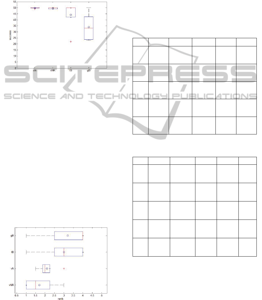
of the algorithms according to the success metrics.
The gbest configuration is clearly the worst
algorithm in the test set under this criterion. The
standard Von Neumann configuration is the most
consistent (in the total 250 runs, it only failed in one
run), but the 99 Von Neumann attains similar
results: in 250 runs it only failed twice.
Figure 1: Rank by success rates. Von Neuammn random
partially connected structure (vNR), Von Neumann (vN),
lbest (lB) and gbest (gB).
A general evaluation of the four topologies
according to fitness, speed and success results in the
following ranking: 99 von Neumann (1.7),
standard von Neumann (2.1), lbest (3.0) and gbest
(3.2). The proposed structure ranks first. Figure 2
shows the boxplot of the ranking.
As demonstrated above, the proposed partially
connected structures are able to improve the
standard configuration and the classical lbest and
gbest topologies. The question that arises now is
what makes these random structures better. The
differences to the standard configuration are the
candidates for explaining the differences: different
average connectivity, dynamic connectivity and
neighborhood, and memory (please remember that a
particle retains a
, even if the informant is no
longer in the neighborhood, until a better pg is
transmitted by a neighbor).
Figure 2: Rank by overall performance.
Some tests with non-memory versions of the
dynamic structures showed that the memory version
performs generally better. However, non-memory
structures do not necessarily perform worst and this
strategy may be useful under higher connectivity
partially connected structures (with Moore
neighborhood, for instance). This study is beyond
the scope of this paper and the main conclusion at
this moment is that the memory scheme is beneficial
for the proposed Von Neumann structure.
Table 8: Moore topologies. Best fitness values averaged
over 50 runs.
f
1
f
2
f
3
f
4
f
5
Moore
2.04e‐41 1.23e+01 6.78e+01 9.98e‐03 1.94e‐04
±2.78e‐41 ±2.28e+01 ±1.54e+01 ±1.42e‐02 ±1.37e‐03
Moore
(7×7)
1.80e‐42 9.51e00 7.61e+01 9.15e‐03 1.55e‐03
±6.81e‐39 ±1.94e+00 ±2.28e+01 ±1.31e‐02 ±3.60e‐03
Moore
(8×8)
7.04e‐41 6.02e00 7.62e+01 1.20e‐02 2.77e‐04
±1.46e‐40 ±1.88e+01 ±2.23e+01 ±1.50e‐02 ±2.66e‐03
Moore
(9×9)
9.08e‐40 1.02e+01 6.86e+01 9.54e‐03 1.17e‐03
±1.26e‐39 ±1.94e+01 ±1.98e+01 ±1.42e‐02 ±3.19e‐03
Moore
(10×10)
9.78e‐39 1.12e+01 6.87e+01 6.61e‐03 5.83e‐04
±1.76e‐38 ±2.16e+01 ±1.79e+01 ±1.03e‐02 ±1.37e‐03
Table 9: Von Neumann topologies. Iterations to a solution
averaged over 50 runs and number of successful runs.
f
1
f
2
f
3
f
4
f
5
Moore
419.58 1092.70 338.78 395.88 295.96
±17.56
(50)
±1209.86
(50)
±427.94
(49)
±28.19
(49)
±263.47
(50)
Moore
(7×7)
410.10 1605.58 250.71 385.45 521.52
±22.29
(50)
±1955.77
(50)
±78.12
(42)
±29.22
(49)
±703.56
(45)
Moore
(8×8)
427.98 1745.70 320.63 396.35 427.15
±17.55
(50)
±1805.28
(50)
±69.971
(45)
±26.88
(49)
±1026.02
(49)
Moore
(9×9)
440.26 2199.04 658.71 405.02 345.38
±21.13
(50)
±2233.83
(50)
±1270.512
(47)
±27.35
(47)
±939.29
(49)
Moore
(10×10)
452.08 1485.10 512.38 418.46 794.18
±17.51
(50)
±1720.67
(50)
±194.09
(47)
±24.96
(50)
±2259.27
(49)
4.2 Moore Neighborhood
Table 8 and Table 9 compare the Moore standard
configuration with partially connected Moore
structures. Table 8 gives the averaged best fitness
found by the swarms, while Table 9 gives, for each
algorithm and each function, the averaged number of
PerformanceandScalabilityofParticleSwarmswithDynamicandPartiallyConnectedGridTopologies
53

iterations required to meet the criterion, and the
number of runs in which the criterion was met.
The Moore dynamic structure with size 7×7, for
instance, is clearly better than the standard
configuration in functions f
1,
f
2
and f
3
, while being
outperformed in function f
5
. However, the structure
with size 9×9 does not improve significantly the
performance in any function, while being
outperformed in f
1
and f
5.
It seems that a sparse
connectivity degrades the performance of the Moore
structure, especially in the convergence speed of the
algorithm.
Table 10: 15. Best fitness values averaged over 50
runs.
f
1
f
2
f
3
f
4
VN
8.06e‐22 6.57e00 1.26e+01 1.46e‐02
±1.09e‐21 ±2.28e+01 ±5.72e00 ±1.70e+02
VN
(9×9)
1.68e‐22 1.73e00 1.50e+01 3.44e‐02
±2.03e‐22 ±3.29e00 ±6.58e00 ±2.73e‐02
Table 11: 15. Iterations to a solution averaged over
50 runs and number of successful runs.
f
1
f
2
f
3
f
4
VN
236.62 491.82 52.84 267.74
±11.12
(50)
±863.31
(49)
±12.41
(50)
±78.55
(46)
VN
(9×9)
233.38 351.82 55.52 297.56
±9.62
(50)
±370.88
(50)
±15.60
(50)
±92.07
(39)
4.3 Scalability
A simple scalability test of the von Neumann
structures was conducted by setting the
dimensionality of the functions
,
,
and
to
15and 60. Like in Section 4.1, two sets of
experiments were conducted. In the first set, the
algorithms were run for a limited amount of
iterations: with 15, 1000 iterations for
and
6000 for
,
and
; with 60, 3000 iterations
for
and 20000 for
,
and
. In the second set
of experiments the algorithms were all run for
20000 iterations or until reaching a stop criterion.
The criteria are as in Section 4.1, except with the
60-dimensional
function, for which the criteria
was set to 300 (because none of the algorithms
could meet the criterion set for the 30 version).
The number of iterations required to meet the
criterion was recorded and averaged over the 50
runs. A success measure was defined as the number
of runs in which an algorithm attains the fitness
value established as the stop criterion.
Results comparing the standard von Neumann
configuration and the 99 partially connected
configuration are in Tables 10-13. With
, the
standard and the partially connected configurations
are statistically equivalent for both 15 and
60. With
, the 99 topology is significantly
better than the standard von Neumann configuration
when 15 and 60. With
, the two
configuration are equivalent for 15 and the
99 topology is significantly better for 60.
Finally, with
, the partially connected 99
topology is worse when 15, but it is statistically
equivalent to the standard topology when 60.
Non-parametric Mann–Whitney U statistical
tests (with 0.05 level of significance) were used. A
version of the algorithm was considered statistically
better if at least one of the measures (average best
solution and average number of iterations to a
solution) was found to be statistically better, while
the other is at least equivalent.
Table 12: 60. Best fitness averaged over 50 runs.
f
1
f
2
f
3
f
4
VN
4.49e‐15 4.67e+01 2.79e+02 4.96e‐03
±3.68e‐15 ±5.51e+01 ±4.91e+01 ±1.04e‐02
VN
(9×9)
5.28e‐15 2.25e+01 2.50e+02 5.55e‐03
±8.54e‐15 ±3.50e+01 ±4.44e+01 ±1.26e‐02
Table 13: 60. Iterations to a solution averaged over
50 runs and number of successful runs.
f
1
f
2
f
3
f
4
VN
1054.24 6047.84 785.52 936.49
±29.11
(50)
±4693.06
(44)
±738.50
(31)
±42.52
(49)
VN
(9×9)
1042.76 6045.90 524.41 933.90
±52.70
(50)
±4264.85
(49)
±143.45
(44)
±56.99
(49)
These results, together with those discussed in
Section 4.1, show that the proposed partially
connected topology scales similarly to the standard
von Neumann topology on
,
and better on
and
. Please note that the 99 topology was used
here, i.e., no tuning of the grid size was done for
optimizing the performance. This particular
configuration is not only consistent throughout the
proposed test set, but also robust to the problem size.
IJCCI2013-InternationalJointConferenceonComputationalIntelligence
54

5 CONCLUSIONS
This paper describes a study on the effects of
alternative population structures on the behavior of
the Particle Swarm Optimization (PSO). Dynamic
and partially connected structures were tested by
placing the particles on a grid of nodes larger than
the swarm size. The particles move randomly on the
grid and the network of information is defined in
each iteration by the particle’s position in the grid
and by its neighborhood.
Von Neumann Structures with growing size were
tested on a classical test set and compared to
standard topologies. The results demonstrate that the
proposed structure performs consistently throughout
the test set, improving the performance of other
topologies in the majority of the scenarios and under
different performance evaluation criteria. The
structure is robust to the ratio between the grid size
and the swarm size and a fixed size with ratio 1:2
performs well on every function. A scalability test
was conducted by varying the dimensionality of four
functions in the test set. The proposed topology
scales similarly to the standard von Neumann
topology in two functions, and better in the two
other functions.
In the future, the test set will include more
functions. Non-random strategies for the movement
based on the fitness and the Euclidean distance
between the particles will also be considered.
ACKNOWLEDGEMENTS
The first author wishes to thank FCT, Ministério da
Ciência e Tecnologia, his Research Fellowship
SFRH/BPD/66876/2009). This work was supported
by FCT PROJECT [PEst-OE/EEI/LA0009/2011],
Spanish Ministry of Science and Innovation project
TIN2011-28627-C04-02, Andalusian Regional
Government P08-TIC-03903 and CEI-BioTIC UGR
project CEI2013-P-14.
REFERENCES
Hseigh, S.-T., Sun, T.-Y, Liu, C.-C., Tsai, S.-J. 2009.
Efficient Population Utilization Strategy for Particle
Swarm Optimizers. IEEE Transactions on Systems,
Man and Cybernetics—part B, 39(2), 444-456.
Kennedy, J., Eberhart, R. 1995. Particle Swarm
Optimization. In Proceedings of IEEE International
Conference on Neural Networks, Vol.4, 1942–1948.
Kennedy, J., Mendes, R., 2002. Population structure and
particle swarm performance. In Proceedings of the
IEEE World Congress on Evolutionary Computation,
1671–1676.
Liang, J. J., Qin, A. K., Suganthan, P. N., Baskar, S.,
2006. Comprehensive learning particle swarm
optimizer for global optimization of multimodal
functions. IEEE Trans. Evolutionary Computation,
10(3), 281–296.
Parsopoulos, K. E., Vrahatis, M. N., 2004. UPSO: A
Unified Particle Swarm Optimization Scheme, Lecture
Series on Computer and Computational Sciences, Vol.
1, Proceedings of the International Conference of
"Computational Methods in Sciences and
Engineering" (ICCMSE 2004), 868-87
Parsopoulos, K. E., Vrahatis, M. N., 2005. Unified Particle
Swarm Optimization in Dynamic Environments.
Lecture Notes in Computer Science (LNCS), Vol.
3449, Springer, 590-599.
T. Peram, K. Veeramachaneni, C. K. Mohan, Fitness-
distance-ratio based particle swarm optimization. In
Proc. Swarm Intell. Symp., 2003, pp. 174–181.
Shi, Y. Eberhart, R. C. 1998. A Modified Particle Swarm
Optimizer. In Proceedings of IEEE 1998 International
Conference on Evolutionary Computation, IEEE
Press, 69–73.
Trelea, I. C. 2003. The Particle Swarm Optimization
Algorithm: Convergence Analysis and Parameter
Selection. Information Processing Letters, 85, 317-
325.
PerformanceandScalabilityofParticleSwarmswithDynamicandPartiallyConnectedGridTopologies
55
