
Application of Mathematical Modelling
for Simulation of Galvanic Corrosion
Vít Jeníček, Martina Pazderová and Linda Diblíková
Aerospace Research and Test Establishment – Testing Laboratories, Beranových 130, Prague, Czech Republic
Keywords: Mathematical Modelling, Galvanic Corrosion, Thin Electrolyte Layer, Polarization.
Abstract: This paper deals with an application of mathematical modelling for simulation of galvanic corrosion. A
programme for simulation of galvanic corrosion in a thin film electrolyte layer is presented. The programme
comprises some mathematical simplifications bringing significant reduction of computational demands and
on the other hand a need of specific form of input data. Necessary background for galvanic corrosion is
mentioned and the simplifications are described as well as the form of input data. An example of measured
input data and their application is shown. Discussion of used assumptions, input data availability and
measuring possibilities of the input data is included.
1 INTRODUCTION
Corrosion is significant problem affecting all
engineering materials and causing technical
problems, safety risks and economical losses.
Prevention or reparations are two different
approaches to restriction of corrosion impacts.
Mathematical modelling is an approach to corrosion
prevention, which enables control of an engineering
structure with regard to corrosion resistivity already
during designing process.
Mathematical model is based on physical
description of solved situation and simulation of
processes taking place in the system needs
appropriate input data. Purpose of this paper is to
define input data for simulation of galvanic
corrosion and conditions under which they are to be
measured. Applicability and limitations due to
employed physical model are shown for presented
corrosion simulation software.
2 GALVANIC CORROSION
Galvanic corrosion is one form of corrosion
occuring when two dissimilar metals are connected
in a presence of an electrolyte. Each metal immersed
into an electrolyte has unique potential called
corrosion potential E
corr
. If two metals are
connected, the potential difference becomes a
driving force for a current flowing between the
metals. The electrical circuit closes through the
electrolyte. The flowing current called corrosion
current I
corr
(or corrosion current density j
corr
if
converted per unit area) causes dissolution of less
noble metal (metal with lower E
corr
). This metal
becomes an anode of an electrochemical corrosion
cell. The metal with higher E
corr
becomes an
cathode. On the cathode, depolarization processes
proceeds which do not cause the dissolution of the
metal. Current flowing between the metal and the
ellectrolyte changes the potential of the metal. The
relation between the current density and the potential
change is represented by polarization curve.
To predict an impact of galvanic corrosion is
difficult because it depends not only on the material
properties but also on the geometry of the
connection and fast, localized degradation can occur.
If more than two materials are connected, the
situation becobes very complex.
3 SIMULATION SOFTWARE
Software BEASY Corrosion Manager (CM BEASY
Ltd., UK) was used for the simulation. The
programme enables to model galvanic corrosion
under thin layer of electrolyte. In this context it
means, that the thickness of the layer covering
modelled structure is much smaller than the
characteristic dimension of solved structure. For
example atmospheric corrosion can be described as
461
Jení
ˇ
cek V., Pazderová M. and Diblíková L..
Application of Mathematical Modelling for Simulation of Galvanic Corrosion.
DOI: 10.5220/0004588504610466
In Proceedings of the 3rd International Conference on Simulation and Modeling Methodologies, Technologies and Applications (SIMULTECH-2013),
pages 461-466
ISBN: 978-989-8565-69-3
Copyright
c
2013 SCITEPRESS (Science and Technology Publications, Lda.)

corrosion in a thin layer of adsorbed moisture or thin
layer of electrolyte corresponds with rainfalls
covering upper parts of an aircraft fuselage.
Under assumption of thin layer of electrolyte,
following steps can be done (Palani 2011) to model
galvanic corrosion.
The schematic depiction of galvanic corrosion
under the thin film is in Figure 1.
Figure 1: Schematic depiction of galvanic corrosion under
a thin film of electrolyte, w«L.
Equation to be solved is the charge conservation
equation in the electrolyte under steady state (1):
0j
(1)
where
xVj
e
is the current density, σ
is the electrolyte conductivity and V
e
(x) is the
electric potential in the electrolyte at point
3
Rx .
The integration domain of the equation (1) is the
volume of the electrolyte.
The boundary conditions for the surface of the
anode and of the cathode are given by equation (2):
Vf
n
V
j
e
n
(2)
where j
n
is the current density flowing through
the surface in normal direction and ΔV is the
polarization potential across the metal/electrolyte
interface. Polarization potential is given by
me
VVV where V
m
is the potential of the
metal. This boundary condition is described by the
corresponding polarization curve for the metal of the
anode and of the cathode respectively. These
polarization curves must be contained in input data
for the simulation.
The boundary conditions for insulating surfaces
are j
n
=0.
In general, it is necessary to solve this problem in
3D. But if the thickness of the electrolyte w is much
smaller than a characteristic dimension of the
problem (see Figure 1), the electrical potential V
e
can be considered as constant in z direction. This
behaviour allows excluding the
zj
z
component from the mathematical formulation of
the problem by direct integration of it along the
thickness w and the equation (1) changes into
equation (3):
VfVw
eDD
22
(3)
where w is the thickness of the electrolyte and
D2
represents two dimensional grad operator
acting on x and y coordinates. The effect of the
charge exchange between the anode and the
electrolyte or the cathode and the electrolyte is
presented as source term and not as a boundary
condition. The dimensionality of the problem is
lowered from three to two.
Even very complex shapes with thin film of
electrolyte can be solved as 2D problem although
this “flat surface” can be twisted in fact. Lowering
of the dimensionality brings furthermore substantial
decrease of the computational demands.
4 INPUTS
Input data for the mathematical modelling are the
geometry of solved structure, the polarization curves
of each included material, conductivity of present
electrolyte and the thickness of the electrolyte layer.
4.1 Geometry
Geometry of solved structure is the basis of
mathematical model. Modelling software BEASY
CM uses universal preprocessor GiD (CIMNE,
Spain), which enables to create a new geometry or to
import an existing geometry in format IGES, DXF,
Parasolid, ACIS, VDA, Rhino, or Shapefile. Because
the corrosion is a matter of a surface of material,
geometry prepared for the simulation of corrosion has
to be composed only of surfaces. For the calculations
the surface is divided into elements by a discretization
mesh. Because the galvanic corrosion takes place in
vicinity of different materials interface, the mesh has
to be thicken in this areas.
4.2 Polarization Curves Measurement
The key input data for the simulation are the
polarization curves. They should be measured under
circumstances similar to those causing galvanic
corrosion. It requests measuring in thin layers of
electrolyte. Thin layer of electrolyte in this context
means layer thinner than 100 μm. Such thin layers
SIMULTECH2013-3rdInternationalConferenceonSimulationandModelingMethodologies,Technologiesand
Applications
462
results in different polarization processes and
different shape of measured polarization curve in
comparison with a bulk electrolyte (Xiao 2012).
Common term in literature is thin electrolyte layer
(TEL).
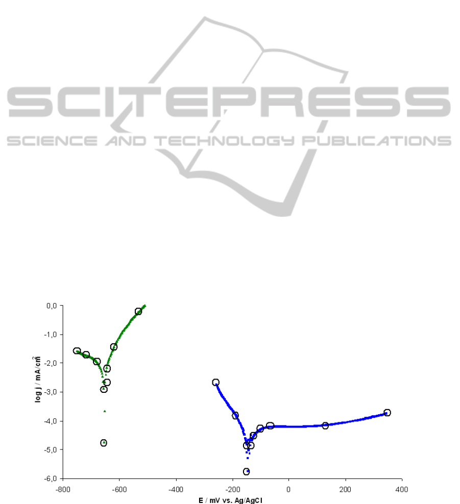
Polarization curves used for modelling of a
structure presented in this paper as an example are
shown in Figure 2. Measured polarization curves are
modified for the use in the programme. A few
discrete points interconnected by lines represent
them in the programme. The points for this
linearization are shown in Figure 2 too.
Factors influencing the shape of measured
polarization curves are the thickness of the layer,
chemical composition of the electrolyte and the
temperature. Software BEASY CM does not solve
processes on the metal/electrolyte interface.
Influence of all mechanisms (thermodynamics and
kinetics of electrochemical reactions) influencing the
resulting shape of the polarization curve has to be
included in the measured curves. In dependence on
different corrosive conditions to be modelled, there
must be accessible a broad database of polarization
curves, covering all corrosive conditions for all
materials.
4.3 Influence of Coatings
A material with a coating can be modelled as a
surface characterized by a new polarization curve.
Another approach is included, to use a polarization
curve of the plain material and the influence of the
coating model by two variables – breakdown factor
and ohmic resistance. This possibility is appropriate
especially for paints.
Breakdown factor indicates the ratio of area
without coating to the total area of a surface. This
definition enables to model damaged coatings.
Default value is set to 1, describing surface with no
coating. Ohmic resistance characterizes the electrical
properties of the coating. Default value is set to 0,
describing surface with no coating as well.
For coatings capable of electrochemical
reactions, typically galvanic coatings, there is a need
to measure a new polarization curve of the material
with the coating.
4.4 Thickness and Conductivity of TEL
Be the layer of electrolyte thicker than 100 μm or
thinner, the thickness of the layer is a part of input
data together with electrical conductivity of the
electrolyte. For a simulation of atmospheric
corrosion very thin adsorbed layers are used with a
thickness in the range 10-100 µm (Yadav 2007). If
water flowing down or stagnant appears, thicker
layers are modelled. The thickness must be
measured, calculated (Palani 2011) or estimated.
Measured thicknesses for typical situations can be
used repeatedly.
Conductivity of the electrolyte depends on the
composition. Aqueous solutions are most common
although an influence of any type of liquid can be
investigated by presented software on principle.
Conductivity of aqueous solution depends on an
amount of dissolved chemicals (salts, gases etc.).
Composition and conductivity of the electrolyte for
typical situations should be analyzed and
consequently it can be estimated on the basis of
similarity.
Figure 2: Measured polarization curves in thin layer of water: mild steel – green, stainless steel – blue.
ApplicationofMathematicalModellingforSimulationofGalvanicCorrosion
463
5 OUTPUTS
Results of the calculation are potential and current
density distribution over the whole surface of solved
structure. Calculated value of current density
represents the normal component of total current.
This is the current flowing between the metal and
the electrolyte, which is the corrosion current. For a
visualization of the results postprocessor GiD is used
again.
Small construction detail was solved to illustrate
the simulation outputs. It is a connection between a
hydraulic cylinder and a landing gear of an aircraft.
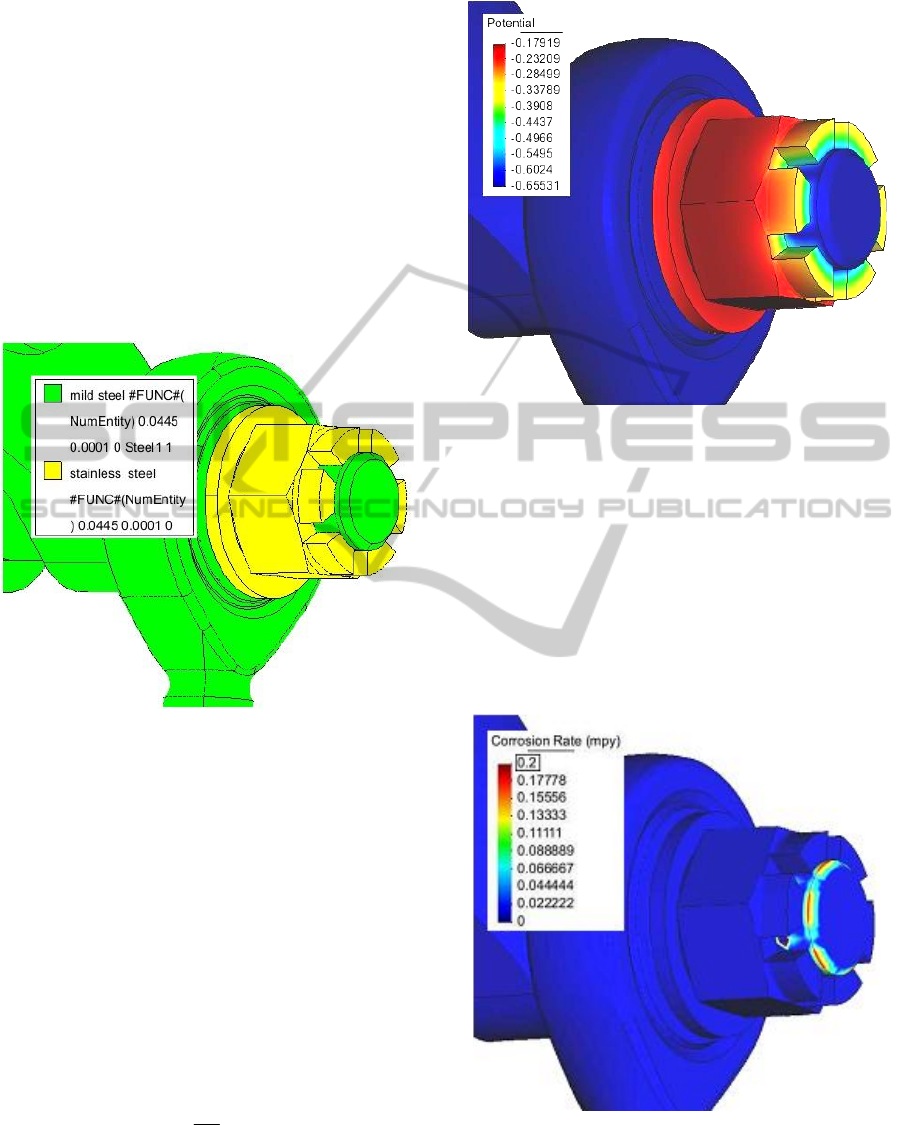
Modelled material composition is shown in Figure 3.
Figure 3: Modelled construction detail and the material
composition.
Modelled distribution of potential in the TEL is
shown in Figure 4. Solved structure includes two
different materials – stainless steel nut and washer
and other parts from mild steel. The stainless steel
has higher E
corr
(is electrochemically more noble)
and the potential of TEL above the nut corresponds
to it. Towards the material interface the potential
lowers and above the mild steel parts far from the
material interface, the potential of TEL is the lowest.
As en improvement, visualization of corrosion
rate was added into the programme. Corrosion rate
CR [mpy] (mils per year) is coupled with calculated
current density by equation 4.
EW
j
KCR
n
1
(4)
where K
1
=327.2 [mm.kg/(A.m.year)] is a
constant including Faraday’s constant and the unit
conversion factor, ρ is the metal density and EW is
equivalent weight, characteristic for each material.
Figure 4: Modelled distribution of potential. Mild steel
parts and stainless steel nut in thin layer of water (100
μm).
Modelled distribution of corrosion rate is shown
in Figure 5. The figure clearly shows that the
electrochemically less noble mild steel corrodes in
the vicinity of the material interface. Distribution of
the corrosion rate is not uniform. The highest
corrosion rate is near the edges of the stainless steel
nut. Material interface between the washer and the
loop of the hydraulic cylinder is not visible in the
figures.
Figure 5: Modelled distribution of CR. Mild steel parts and
stainless steel nut in thin layer of water (100 μm).
Another quantity characterising the intensity of a
corrosion attack is mass loss rate MLR [g/(day.m
2
)]
satisfying equation 5.
SIMULTECH2013-3rdInternationalConferenceonSimulationandModelingMethodologies,Technologiesand
Applications
464

EWjKMLR
n2
(5)
where K
2
=0.8953 [g/(A.day)] is a constant including
Faraday’s constant and the unit conversion factor.
6 DISCUSSION
6.1 Assumptions Discussion
The main assumption used in BEASY CM is the
assumption of the thin layer of electrolyte. This
assumption enables to treat the volume of the
electrolyte as a layer characterized only by the value
of its sheet resistance. Currents flowing through the
layer in the longitudinal direction cause the
continuous distribution of the potential. Mutual
interaction between the electrolyte and the material
of investigated structure is controlled by the
polarization behaviour of the material and is
presented in the electrolyte as a source of current
(positive or negative). This current flows in normal
direction to the surface, represents the corrosion
current and is controlled by the local electrolyte
potential and corresponding polarization curve.
Flow of the current in the volume of the
electrolyte is not solved. This assumption brings
mentioned lowering of computational demand, but
has to be taken into account, when a real situation is
studied. Qualified decision has to be made, if it is
possible to model the situation by BEASY CM or
not. Critical in this case are fine details with
different materials covered by relatively thick layer
of electrolyte. This situation is not common in a case
of atmospheric corrosion, because the thickness of
adsorbed moisture is about 10 – 100 μm. Caution is
needed, when a corrosion in thicker layers is
modeled, for example the layer of stagnant water
covering a part of a car chassis.
Polarization curves are used directly during the
calculation as a binding condition between the
potential of the electrolyte and the flowing corrosion
current. BEASY CM does not solve the mechanisms
of polarization. Therefore, the polarization curves
have to be measured under conditions as close as
possible to those prevailing during the exposition to
the corrosive environment. Factors influencing the
resulting shape of polarization curve are
temperature, composition of the electrolyte,
composition of surrounding atmosphere and the
thickness of the electrolyte layer. For the simulation
of galvanic corrosion by BEASY CM it is necessary
to have a database of polarization curves for all
included materials covering broad spectrum of
measuring conditions or to have a possibility to
arbitrarily measure the curves of included materials
for every specific situation which is to be simulated.
6.2 Input Data Discussion
Because there is no comprehensive database of
polarization data for materials in TEL in the
literature, the measuring of polarization curves is an
essential part of using BEASY CM. Because of large
serial resistance of the TEL, the measuring in the
thin layer requires special techniques. Contactless
measurement (Stratmann, 1990) or a special type of
corrosion cell (Liu, 2010) are most frequently
mentioned in the literature. There is a possibility to
measure polarization curves in TEL in Testing
Laboratories of Aerospace Research and Test
Establishment. The technique is under permanent
development and the minimum achievable thickness
is decreasing.
As mentioned above, the layer of the electrolyte
is characterized with its sheet resistance. This value
is given by a conductivity of the electrolyte and the
thickness of the layer. Factors influencing the
conductivity of an electrolyte are temperature and
the composition of the electrolyte.
The main issue during solving a real situation by
BEASY CM is to determine the thickness of the
electrolyte layer, the composition of the electrolyte
and consequently its conductivity and the
appropriate polarization curve.
7 CONCLUSIONS
Philosophy of a programme BEASY CM for
mathematical modelling of galvanic corrosion was
introduced. As a special tool for modelling of
galvanic corrosion in TEL, the programme uses
mathematical simplifications resulting from physical
description of the situation. The programme solves
the galvanic corrosion as a 2D problem. This
simplification must be considered as a limiting
factor, when decision should be made, if the
software can be used for modelling of particular
situation or not.
On the other hand the programme need special,
precisely measured input data. This data are
polarization curves measured in TEL and the
measuring conditions should cover a broad spectrum
of corrosive environments. The other disputable
variables are the thickness of TEL and the electrical
conductivity of the electrolyte. It is advisable to have
a database of the thicknesses and electrolyte
ApplicationofMathematicalModellingforSimulationofGalvanicCorrosion
465

conductivities for typical corrosive environments.
REFERENCES
Liu, W., Cao, F., Chen, A., Chang, L., Zhang, J. and Cao,
C., 2010. Corrosion behaviour of AM60 magnesium
alloys containing Ce or La under thin electrolyte
layers. Part 1: Microstructural characterization and
electrochemical behaviour. Corrosion Science,
February 2010, Vol.52, No.2, pp 627-638
Palani, S., Hack, T., Perrata, A., Adey, R., Baynham, J.
and Lohner, H., 2011. Modeling approach for galvanic
corrosion protection of multimaterial aircraft
structures. BEASY Software and Services.
http://www.beasy.com/news/pdfs/Aircraft_Structure_
Corrosion_DOD_2011.pdf (accessed May 17, 2013)
Stratmann, M. and Streckel, H., 1990. On the atmospheric
corrosion of metals which are covered with thin
electrolyte layers I-III. Corrosion Science, June/July
1990, Vol.30, No.6/7, pp 681-734
Xiao, K., Dong, C. F., Luo, H., Liu, Q., and Li, X. G.,
2012. Investigation on the Electrochemical Behaviour
of Copper Under HSO
3
-
-containing Thin Electrolyte
Layers. International Journal of Electrochemical
Science, August 2012, Vol.7, No.8, pp 7503-7515
Yadav, A. P., Katayama, H., Noda, K., Masuda, H.,
Nishikata, A. and Tsuru, T., 2007. Effect of Al on the
galvanic ability of Zn-Al coating under thin layer of
electrolyte. Electrochimica Acta, February 2007,
Vol.52, No.7, pp 2411-2422
SIMULTECH2013-3rdInternationalConferenceonSimulationandModelingMethodologies,Technologiesand
Applications
466
