Optimized Eigenstructure Assignment
Ngoc Minh Dao
1,2
, Dominikus Noll
1
and Pierre Apkarian
3
1
Institut de Math
´
ematiques, Universit
´
e de Toulouse, Toulouse, France
2
Department of Mathematics and Informatics, Hanoi National University of Education, Hanoi, Vietnam
3
ONERA, Department of System Dynamics, Toulouse, France
Keywords:
Eigenstructure Assignment, Output Feedback Control, Nonlinear Optimization, Hankel Norm.
Abstract:
This paper considers the problem of eigenstructure assignment for output feedback control. We introduce a
new method for partial eigenstructure assignment, which allows to place the eigenelements (λ
i
,v
i
,w
i
) simul-
taneously. This is possible by a combination of linear algebra and nonlinear optimization techniques. The
advantage of the new approach is illustrated through the control of a launcher in atmospheric flight.
1 INTRODUCTION
Eigenstructure assignment has been shown to be a
powerful controller design tool in the aerospace sec-
tor and in other high technology fields. This approach
aims at shaping the responses of the closed-loop sys-
tem to certain input signals by way of three mecha-
nisms. The placement of closed-loop modes in order
to arrange satisfactory decay rates, the choice of suit-
able eigenvectors to shape specific responses, and the
possibility to decide to what extent initial conditions
contribute to these responses.
In this paper we focus on the design of output
feedback control laws, where only partial eigenstruc-
ture assignment or pole placement can be expected.
Here the standard approach to first selecting a par-
tial set of closed-loop modes and then using the re-
maining degrees of freedom to shape the correspond-
ing closed-loop eigenvectors, may fail to stabilize the
system in closed-loop, as the remaining closed-loop
modes cannot be influenced directly.
Consider a linear time-invariant system described
by the equations
˙x = Ax + Bu
y = Cx
(1)
with x ∈ R
n
, u ∈ R
m
and y ∈ R
p
. Given a self-
conjugate set Λ = {λ
1
,.. .,λ
p
} ⊂ C
−
, partial pole
placement consists in computing a static output feed-
back control law u = Ky for (1) such that λ
1
,.. .,λ
p
become eigenvalues of the closed-loop system
˙x = (A + BKC)x.
As is well-known, solving the set of linear equations

A −λ
i
I
n
B


v
i
w
i

= 0,
with v
i
∈ R
n
, w
i
∈ R
m
, i = 1,. .., p leads to a control
law
K = [w
1
,.. .,w
p
](C [v
1
,.. .,v
p
])
−1
(2)
with the desired closed-loop modes, provided the
v
i
are chosen in such a way that the p × p matrix
C [v
1
,.. .,v
p
] is invertible, i.e., if span{v
1
,.. .,v
p
}∩
ker(C) = {0}.
In case m > 1 it is possible to achieve more. One
may then shape the v
i
, respectively w
i
, e.g. by arrang-
ing v
i j
= 0 or w
ik
= 0 for certain j,k. This can be
expressed by linear equations

A −λ
i
I
n
B
M
i
N
i

v
i
w
i

=

0
r
i

, (3)
where M
i
∈ R
m
i
×n
, N
i
∈ R
m
i
×m
, r
i
∈ R
m
i
, m
i
> 0,
i = 1,. .., p, leaving at least one degree of freedom.
This is referred to as partial eigenstructure assign-
ment.
The traditional approach in eigenstructure assign-
ment consists in choosing the set Λ ⊂ C
−
, and then
adding the desired structural constraints on the eigen-
vectors v
i
,w
i
, using the remaining degrees of free-
dom. However, fixing the λ
i
may be too restrictive for
the second step, because we should not forget that par-
tial eigenvalue placement does not guarantee stabil-
ity in closed-loop, so that some post-processing may
be required, which often leads to unsatisfactory trial-
and-error. Greater flexibility in the design could be
307
Minh Dao N., Noll D. and Apkarian P..
Optimized Eigenstructure Assignment.
DOI: 10.5220/0004594903070314
In Proceedings of the 10th International Conference on Informatics in Control, Automation and Robotics (ICINCO-2013), pages 307-314
ISBN: 978-989-8565-70-9
Copyright
c
 2013 SCITEPRESS (Science and Technology Publications, Lda.)

achieved by moving (λ
i
,v
i
,w
i
) simultaneously. This
may in particular be achieved by optimization if (3) is
used as a constraint, under which closed-loop stability
or performance are improved.
2 PROBLEM STATEMENT
We discuss the problem of partial eigenstructure as-
signment for a static feedback output controller. Con-
sider a linear time-invariant plant P in standard form
P :
˙x = Ax + B
1
w + Bu
z = C
1
x + D
11
w + D
12
u
y = Cx + D
21
w + D
22
u
where x ∈R
n
is the state vector, u ∈ R
m
the vector of
control inputs, w ∈ R
m
1
the vector of exogenous in-
puts, y ∈ R
p
the vector of measurements and z ∈ R
p
1
the controlled or performance vector. Assuming with-
out loss that D
22
= 0, let u = Ky be a static output
feedback control law for the open-loop plant P, and
let T
wz
(K) denote the closed-loop performance chan-
nel w →z. Then T
wz
(K) has the state-space represen-
tation
˙x = (A + BKC)x +(B
1
+ BKD
21
)w
z = (C
1
+ D
12
KC)x +(D
11
+ D
12
KD
21
)w.
Given a self-conjugate eigenvalues set
Λ
0
= {λ
0
1
,.. .,λ
0
p
} and tolerances δ
i
, we consider the
optimization program
minimize kT
wz
(K)k
subject to

A −λ
i
I
n
B
M
i
N
i

v
i
w
i

=

0
r
i

|λ
i
−λ
0
i
| 6 δ
i
,i = 1,.. ., p
K = K(λ, v,w) as in (2)
(4)
where λ
0
i
are nominal closed-loop pole positions and
(3) as above conveys additional structural constraints
on v
i
,w
i
. This is now a parametrization of the con-
trol law (2) in the sense of structured synthesis intro-
duced in (Apkarian and Noll, 2006). The cost func-
tion kT
wz
(K)k in (4) may now be used to enhance
stability and to achieve additional performance or ro-
bustness specifications of the design.
Standard choices of k · k include the H
∞
-norm
k·k
∞
, the H
2
-norm k·k
2
or the Hankel norm k·k
H
, to
which special attention will be given here. One gen-
erally expects that kT
wz
(K)k < ∞ implies closed-loop
stability, but should this fail, it is possible to add a
stability constraint c(λ, v,w) = α(A + BKC) + ε 6 0
to the cast (4), where ε > 0 is some small threshold,
and where we recall the definition of the spectral ab-
scissa of a matrix
α(M) = max{Re(λ) : λ eigenvalue of M}.
Altogether, we now establish the following algorithm
for partial eigenstructure assignment.
3 HANKEL NORM AND ITS
CLARKE SUBGRADIENTS IN
CLOSED-LOOP
Consider a stable LTI system
G :
˙x = Ax +Bw
z = Cx
with state x ∈ R
n
, input w ∈ R
m
, and output z ∈ R
p
.
If we think of w(t) as an excitation at the input which
acts over the time period t 6 T , then the ring of the
system after the excitation has stopped at time T is
z(t) for t > T . If signals are measured in the energy
norm, this leads to the definition of the Hankel norm
of the system G:
kGk
H
= sup
(

Z
∞
T
z
>
zdt

1/2
: z = Gw,
Z
T
0
w
>
wdt 6 1,w(t) = 0 for t > T > 0

.
Algorithm 1: Optimized eigenstructure assignment.
Input: Nominal modal set Λ
0
= {λ
0
1
,.. .,λ
0
p
} with
distinct λ
0
i
.
Output: Optimal modal set Λ = {λ
1
,.. .,λ
p
}, v
i
,w
i
,
and K
∗
.
1: Nominal assignment. Perform standard eigen-
structure assignment based on Λ
0
and struc-
tural constraints M
i
,N
i
. Obtain nominal eigen-
vectors v
0
i
, w
0
i
, i = 1,..., p. Assure that
C[v
0
1
,.. .,v
0
p
] is invertible and obtain nominal
K
0
=

w
0
1
,.. .,w
0
p

C

v
0
1
,.. .,v
0
p

−1
.
2: Stability and performance. If K
0
assures
closed-loop stability and performance kT
wz
(K
0
)k,
stop the algorithm. Otherwise, goto step 3.
3: Tolerances. Allow tolerances |λ
i
− λ
0
i
| 6 δ
i
,
i = 1,... , p.
4: Parametric assignment. Solve the optimization
program
min kT
wz
(K)k
s.t.

A −λ
i
I
n
B
M
i
N
i

v
i
w
i

=

0
r
i

|λ
i
−λ
0
i
| 6 δ
i
,i = 1,.. ., p.
K = [w
1
,.. .,w
p
](C [v
1
,.. .,v
p
])
−1
K closed-loop stabilizing
(5)
using (λ
0
,v
0
,w
0
) as initial seed.
5: Synthesis. Return optimal Λ = {λ
1
,.. .,λ
p
},
v
i
,w
i
, and K
∗
.
ICINCO2013-10thInternationalConferenceonInformaticsinControl,AutomationandRobotics
308

The Hankel norm can be understood as measuring
the tendency of a system to store energy, which is later
retrieved to produce undesired noise effects known as
system ring. Minimizing the Hankel norm kT
wz
(K)k
H
therefore reduces the ringing in the system.
In order to solve program (5) we will have to com-
pute function values and subgradients of the function
f (x) = kT
wz
(K(x))k
2
H
, where x represents the tunable
parameters x = (λ,v,w). Introducing the notation
A
c
= A + BKC, B
c
= B
1
+ BKD
21
,
C
c
= C
1
+ D
12
KC, D
c
= D
11
+ D
12
KD
21
for the closed-loop, and assuming for the time being
that D
c
= D
11
does not explicitly depend on K, a hy-
pothesis which can be arranged e.g. by the standard
assumption that D
12
= 0 or D
21
= 0, we have
f (x) = kT
wz
(K(x))k
2
H
= λ
1
(X(x)Y (x)),
where λ
1
denotes the maximum eigenvalue of a sym-
metric or Hermitian matrix, and X(x) and Y (x) are the
controllability and observability Gramians that can be
obtained from the Lyapunov equations
A
c
X +X A
>
c
+ B
c
B
>
c
= 0, (6)
A
>
c
Y +YA
c
+C
>
c
C
c
= 0. (7)
Notice that despite the symmetry of X and Y the prod-
uct XY needs not be symmetric, but stability of A
c
in
closed-loop guarantees X  0, Y  0 in (6), (7), so
that we can write
λ
1
(XY ) = λ
1
(X
1
2
Y X
1
2
) = λ
1
(Y
1
2
XY
1
2
),
which brings us back in the realm of eigenvalue the-
ory of symmetric matrices.
Let M
n,m
be the space of n × m matrices,
equipped with the corresponding scalar product
hX,Y i = Tr(X
>
Y ), where X
>
and Tr(X ) are respec-
tively the transpose and the trace of matrix X . We
denote by S
m
the space of m ×m symmetric matrices
and define
B
m
:= {X ∈ S
m
: X  0, Tr(X) = 1}.
Setting Z := X
1
2
Y X
1
2
,Z
i
(x) := ∂Z(x)/∂x
i
and taking
Q to be a matrix whose columns form an orthonor-
mal basis of the eigenspace of dimension ν associated
with λ
1
(Z), then according to (Overton, 1992, Theo-
rem 3), the Clarke subdifferential of f at x consists of
all subgradients g
U
of the form
g
U
= (Tr(Z
1
(x)
>
QU Q
>
),.. .,Tr(Z
n
x
(x)
>
QU Q
>
))
>
,
where U ∈B
ν
, and n
x
is the number of coordinates of
x. On the other hand, denoting by D
K
F the derivate
of F with respect to K, we have
Z
i
(x) = D
K
Z(x)K
i
(x)
= ϕ
i
Y X
1
2
+ X
1
2
ψ
i
X
1
2
+ X
1
2
Y ϕ
i
, (8)
where K
i
(x) := ∂K(x)/∂x
i
, ϕ
i
:= D
K
X
1
2
K
i
(x),
ψ
i
:= D
K
Y K
i
(x). From (6) and (7), and on putting
φ
i
:= D
K
XK
i
(x), we obtain
A
c
φ
i
+ φ
i
A
>
c
= −BK
i
(x)CX −X(BK
i
(x)C)
>
−BK
i
(x)D
21
B
>
c
−B
c
(BK
i
(x)D
21
)
>
, (9)
A
>
c
ψ
i
+ ψ
i
A
c
= −(BK
i
(x)C)
>
Y −Y BK
i
(x)C
−(D
12
K
i
(x)C)
>
C
c
−C
>
c
D
12
K
i
(x)C, (10)
by using the fact that D
K
A
c
K
i
(x) = BK
i
(x)C,
D
K
B
c
K
i
(x) = BK
i
(x)D
21
, D
K
C
c
K
i
(x) = D
21
K
i
(x)C.
Since X
1
2
X
1
2
= X,
X
1
2
ϕ
i
+ ϕ
i
X
1
2
= φ
i
. (11)
Altogether, we have the following Algorithm 2 to
compute subgradients of f at x.
Algorithm 2: Computing subgradients.
Input: x ∈ R
n
x
. Output: g ∈∂ f (x).
1: Compute K
i
(x) = ∂K(x)/∂x
i
,i = 1,..., n
x
and
X,Y solutions of (6), (7), respectively.
2: Compute X
1
2
and Z = X
1
2
Y X
1
2
.
3: For i = 1,. .., n
x
compute φ
i
and ψ
i
solutions of
(9) and (10), respectively.
4: For i = 1, ... ,n
x
compute ϕ
i
solution of (11) and
Z
i
(x) using (8).
5: Determine a matrix Q whose columns form an or-
thonormal basis of the eigenspace of dimension ν
associated with λ
1
(Z).
6: Pick U ∈ B
ν
, and return
(Tr(Z
1
(x)
>
QU Q
>
),.. .,Tr(Z
n
x
(x)
>
QU Q
>
))
>
,
a subgradient of f at x.
4 PROXIMITY CONTROL
ALGORITHM FOR
NON-SMOOTH FUNCTIONS
We describe here our algorithm to solve program (5).
More generally, we consider an abstract constrained
optimization program of the form
minimize f (x)
subject to c(x) 6 0
(12)
where x ∈R
n
x
is the decision variable, and f and c are
locally Lipschitz but potentially non-smooth and non-
convex functions. Expanding on an idea in (Polak,
1997, Section 2.2.2), we use a progress function at
the current iterate x,
F(·,x) = max{f (·) − f (x) −νc(x)
+
,c(·) −c(x)
+
},
OptimizedEigenstructureAssignment
309

where c(x)
+
= max{c(x),0}, and ν > 0 is a fixed pa-
rameter. It is easy to see that F(x,x) = 0, where ei-
ther the left branch f (·) − f (x) −νc(x)
+
or the right
branch c(·) −c(x)
+
in the expression of F(·,x) is ac-
tive at x, i.e., attains the maximum, depending on
whether x is feasible for (12) or not. If x is infeasible,
meaning c(x) > 0, then the right hand term in the ex-
pression of F(·,x) is active at x, whereas the left hand
term equals −νc(x) < 0 at x. Reducing F(·,x) below
its value 0 at the current x therefore reduces constraint
violation. If x is feasible, meaning c(x) 6 0, then the
left hand term in F(·,x) becomes dominant, so reduc-
ing F(·,x) below its current value 0 at x now reduces
f , while maintaining feasibility, and where the true
optimization of f takes place.
Observe that if x
∗
is a local minimum of program
(12), it is also a local minimum of F(·,x
∗
), and then
0 ∈ ∂
1
F(x
∗
,x
∗
). The symbol ∂
1
here stands for the
Clarke subdifferential with respect to the first vari-
able. Indeed, if x
∗
is a local minimum of (12) then
c(x
∗
) 6 0, and so for y in a neighborhood of x
∗
we
have
F(y,x
∗
) = max{f (y) − f (x
∗
),c(y)}
> f (y) − f (x
∗
) > 0 = F(x
∗
,x
∗
).
This implies that x
∗
is a local minimum of F(·,x
∗
),
and therefore 0 ∈∂
1
F(x
∗
,x
∗
). We now present Algo-
rithm 3 for computing solutions of program (5).
Convergence theory of iterative algorithm 3 is dis-
cussed in (Gabarrou et al., 2013; Noll, 2010) and
based on these results, we can prove the following
theorem.
Theorem 1. Assume that functions f and c in pro-
gram (12) are lower-C
1
and satisfy the following con-
ditions:
(i) f is weakly coercive on the constraint set
Ω = {x ∈ R
n
x
: c(x) 6 0} in the sense that if
x
j
∈ Ω and kx
j
k → ∞, then f (x
j
) is not mono-
tonically decreasing.
(ii) c is weakly coercive in the sense that if kx
j
k→ ∞,
then c(x
j
) is not monotonically decreasing.
Then the sequence x
j
of serious iterates generated
by Algorithm 3 is bounded, and every accumulation
point x
∗
of the x
j
satisfies 0 ∈ ∂
1
F(x
∗
,x
∗
). 
Notice that f = k·k
2
H
◦G(·) is a composite func-
tion of a semi-norm and a smooth mapping x 7→G(x),
which implies that it is lower-C
2
, and therefore also
lower-C
1
in the sense of (Rockafellar and Wets, 1998,
Definition 10.29). Theoretical properties of the spec-
tral abscissa c(x), used in the constraint, have been
studied in (Burke and Overton, 1994). Lower C
2
-
functions cover the preponderant part of non-smooth
functions encountered in applications. Convergence
Algorithm 3: Proximity control with downshift.
Parameters: 0 < γ <
e
γ < 1,0 < γ < Γ < 1,0 < q < ∞,
0 < c < ∞.
1: Initialize outer loop. Choose initial iterate x
1
and matrix Q
1
= Q
>
1
with −qI  Q
1
 qI. Ini-
tialize memory control parameter τ
]
1
such that
Q
1
+ τ
]
1
I  0. Put j = 1.
2: Stopping test. At outer loop counter j, stop if
0 ∈ ∂
1
F(x
j
,x
j
). Otherwise, goto inner loop.
3: Initialize inner loop. Put inner loop counter
k = 1, initialize τ
1
= τ
]
j
, and build initial work-
ing model F
1
(·,x
j
) using matrix Q
j
.
4: Trial step generation. Compute
y
k
= argminF
k
(y,x
j
) +
τ
k
2
ky −x
j
k
2
.
5: Acceptance test. If
ρ
k
=
F(y
k
,x
j
)
F
k
(y
k
,x
j
)
> γ,
put x
j+1
= y
k
(serious step), quit inner loop and
goto step 8. Otherwise (null step), continue inner
loop with step 6.
6: Update working model. Generate a cutting
plane m
k
(·,x
j
) = a
k
+ g
>
k
(·−x
j
) at null step y
k
and counter k using downshifted tangents. Com-
pute aggregate plane m
∗
k
(·,x
j
) = a
∗
k
+g
∗>
k
(·− x
j
)
at y
k
, and then build new working model
F
k+1
(·,x
j
).
7: Update proximity control parameter. Compute
secondary control parameter
e
ρ
k
=
F
k+1
(y
k
,x
j
)
F
k
(y
k
,x
j
)
and put
τ
k+1
=
(
τ
k
if
e
ρ
k
<
e
γ,
2τ
k
if
e
ρ
k
>
e
γ.
Increase inner loop counter k and loop back to
step 4.
8: Update Q
j
and memory element. Update ma-
trix Q
j
→ Q
j+1
respecting Q
j+1
= Q
>
j+1
and
−qI  Q
j+1
 qI. Then store new memory el-
ement
τ
]
j+1
=
(
τ
k
if ρ
k
< Γ,
1
2
τ
k
if ρ
k
> Γ.
Increase τ
]
j+1
if necessary to ensure
Q
j+1
+ τ
]
j+1
I  0. Increase outer loop counter j
and loop back to step 2.
ICINCO2013-10thInternationalConferenceonInformaticsinControl,AutomationandRobotics
310

theory for even larger classes of non-smooth functions
can be found in (Noll, 2010; Noll et al., 2008).
Corollary 1. Under the hypotheses of the theorem,
every accumulation point of the sequence of serious
iterates generated by Algorithm 3 is either a criti-
cal point of constraint violation, or a Karush-Kuhn-
Tucker point of program (12).
Proof. Suppose x
∗
is an accumulation point of the se-
quence of serious iterates generated by Algorithm 3.
Then 0 ∈ ∂
1
F(x
∗
,x
∗
) due to Theorem 1. By using
(Clarke, 1981, Proposition 9) (see also (Clarke, 1983,
Proposition 2.3.12)), there exist constants λ
0
,λ
1
such
that
0 ∈ λ
0
∂ f (x
∗
) + λ
1
∂c(x
∗
),
λ
0
> 0, λ
1
> 0, λ
0
+ λ
1
= 1.
If c(x
∗
) > 0 then ∂
1
F(x
∗
,x
∗
) = ∂c(x
∗
), and there-
fore 0 ∈ ∂c(x
∗
), that is, x
∗
is a critical point of con-
straint violation. In the case of c(x
∗
) 6 0, if x
∗
is not
a Karush-Kuhn-Tucker point of (12), then we must
have λ
0
= 0, and so 0 ∈ ∂c(x
∗
). We deduce that x
∗
is either a critical point of constraint violation, or a
Karush-Kuhn-Tucker point of program (12).
In the absence of convexity, proving convergence
to a single Karush-Kuhn-Tucker point is generally out
of reach, but the following result gives nonetheless a
satisfactory answer for stopping of the algorithm.
Corollary 2. Under the hypotheses of the theorem,
for every ε > 0 there exists an index j
0
(ε) ∈ N such
that every j > j
0
(ε), x
j
is within ε-distance of the set
L = {x
∗
∈ R
n
x
: 0 ∈∂
1
F(x
∗
,x
∗
)}.
Proof. Since our algorithm assures always that
x
j
− x
j+1
→ 0, by using Ostrowski’s theorem (Os-
trowski, 1973, Theorem 26.1), the set of limit point
L of the sequence x
j
is either singleton or a com-
pact continuum. Our construction then assures con-
vergence of x
j
to the limiting set L in the sense of the
Hausdorff distance. For the details we refer to (Noll,
2012).
5 A SMOOTH RELAXATION OF
HANKEL NORM
This section is motivated by (Nesterov, 2007), which
gives a fine analysis of the convex bundle method
in situations where the objective f (x) has the spe-
cific structure of a max-function, including the case of
a convex maximum eigenvalue function. Nesterov’s
findings indicate that for a given precision, such pro-
grams may be solved with lower algorithmic com-
plexity using smooth relaxations. While these re-
sults are a priori limited to the convex case, it may
be interesting to apply this idea as a heuristic in the
non-convex situation. More precisely, we can try
to solve problem (5), (12) by replacing the function
f (x) = λ
1
(Z(x)) by its smooth approximation
f
µ
(x) := µln
n
∑
i=1
e
λ
i
(Z(x))/µ
!
,
where µ > 0 is a tolerance parameter, n is the order of
matrix Z, and where λ
i
denotes the ith eigenvalue of a
symmetric or Hermitian matrix. Then
∇ f
µ
(Z) =
n
∑
i=1
e
λ
i
(Z)/µ
!
−1
n
∑
i=1
e
λ
i
(Z)/µ
q
i
(Z)q
i
(Z)
>
,
with q
i
(Z) the ith column of the orthogonal matrix
Q(Z) from the eigendecomposition of symmetric ma-
trix Z = Q(Z)D(Z)Q(Z)
>
. We obtain
∇ f
µ
(x) =
(Tr(Z
1
(x)
>
∇ f
µ
(Z)), ... ,Tr(Z
n
x
(x)
>
∇ f
µ
(Z)))
>
.
On the other hand,
f (x) 6 f
µ
(x) 6 f (x) + µln n.
Therefore, to find an ε-solution
¯
x of problem (12), we
find an
ε
2
-solution of the smooth problem
minimize f
µ
(x)
subject to c(x) 6 0
(13)
with µ =
ε
2lnn
. Here we use this idea to initialize the
non-smooth algorithm 3. The smoothed problem (13)
can be solved using standard NLP software.
6 LAUNCHER IN ATMOSPHERIC
FLIGHT
In this section we apply Algorithm 1 to design a
MIMO PI controller for a satellite launcher in atmo-
spheric flight. The linear model is described by
˙x = Ax +Bu
y = Cx
(14)
OptimizedEigenstructureAssignment
311

where
A =











Z
w
Z
q
+U
0
Z
θ
Z
v
0 Z
ψ
Z
p
Z
φ
M
w
M
q
0 0 M
r
0 M
p
0
0 T
q
0 0 T
r
0 0 0
Y
w
0 Y
θ
Y
v
Y
r
Y
ψ
Y
p
Y
φ
0 N
q
0 N
v
N
r
0 N
p
0
0 P
q
0 0 P
r
0 0 0
0 L
q
0 0 L
r
0 L
p
0
0 F
q
0 0 F
r
0 1 0











,
B =


Z
βz
M
βz
0 0 0 0 0 0
0 0 0 Y
βy
N
βy
0 0 0
0 0 0 0 0 0 L
βr
0


>
,
and numerical data in A,B are given in the Appendix.
The state vector x = [w q θ v r ψ p φ]
>
∈R
8
regroups
w = vertical velocity (m/s),
q = pitch rate (deg/s),
θ = pitch angle (deg),
v = lateral velocity (m/s),
r = yaw rate (deg/s),
ψ = yaw angle (deg),
p = roll rate (deg/s),
φ = roll angle (deg).
The control signal is defined as u = [β
z
β
y
β
r
]
>
∈ R
3
with
β
z
= deflection of pitch nozzle actuator (deg),
β
y
= deflection of yaw nozzle actuator (deg),
β
r
= deflection of roll nozzle actuator (deg).
The vector of measurements is
y = [q θ r ψ p φ]
>
∈ R
6
. The model has been
obtained from linearization of the nonlinear equa-
tions (McLean, 1990) about a steady state flight
point
θ
0
= 8.38
◦
, ψ
0
= 3.48
◦
, φ
0
= 11.99
◦
,
U
0
= 88.11 m/s, v
0
= 0.678 m/s, w
0
= −1.965 m/s,
p
0
= −0.0006 rad/s, q
0
= 0.0026 rad/s,
r
0
= 0.0046 rad/s,
the procedure being explained in (Greensite, 1970).
The control law specifications include
• Decoupling of the 3 axes (θ,q), (ψ,r), and (φ, p).
• Well-damped responses to set-points in θ, ψ, and
φ.
• Settling times around 2.5 seconds.
We use a set-point tracking control architecture with
MIMO PI feedback as in Figure 1. Tunable matrix
gains are therefore K
P
and K
I
.
+
−
!
K
I
G
launcher
K
P
H
selector
w
y
uc
v
e
d
+
−
w
ref
.
1
Figure 1: Control architecture with MIMO PI-controller.
For simulation we use the closed-loop transfer
function T
w
ref
→y
(K) that requires the plant P
sim
:


y(s)
y(s)
d(s)


=


0 G(s)
0 G(s)
s
−1
I
3
−s
−1
HG(s)



w
ref
(s)
u(s)

,
which is in closed-loop with the static output feed-
back control law
K : u(s) =

−K
P
K
I


y(s)
d(s)

.
Here w = (θ,ψ,φ) = Hy, d = s
−1
(w
ref
−w), and
H =


0 1 0 0 0 0
0 0 0 1 0 0
0 0 0 0 0 1


.
It is also convenient to introduce a second perfor-
mance plant P
perf
to assess the closed-loop channel
T
w
ref
→e
(K). This requires


e(s)
y(s)
d(s)


=


I
3
−HG(s)
0 G(s)
s
−1
I
3
−s
−1
HG(s)



w
ref
(s)
u(s)

along with the same control structure K.
For pole placement respectively eigenstructure as-
signment we shall therefore use
A
a
=

A 0
−HC 0

,B
a
=

B
0

,C
a
=

C 0
0 I
3

,
and the control law is defined by K
a
= W (C
a
V )
−1
,
K
a
= [−K
P
K
I
], where
W = [w
1
... w
9
], V = [v
1
... v
9
],
[A
a
−λ
i
I
11
|B
a
]

v
i
w
i

= 0.
The pole placement is performed by using refer-
ence values of the second order system ξ and ω. We
choose the desired damping ξ =
√
2
2
, and frequencies
ω
1
= 2.1, ω
2
= 2.2, ω
3
= 1.8,
ICINCO2013-10thInternationalConferenceonInformaticsinControl,AutomationandRobotics
312

which leads to the nominal modal set
Λ = {λ
0
1
,.. .,λ
0
9
}, where
λ
0
1,2
= −ω
1

ξ ± j
q
1 −ξ
2

,
λ
0
3,4
= −ω
2

ξ ± j
q
1 −ξ
2

,
λ
0
5,6
= −ω
3

ξ ± j
q
1 −ξ
2

,
λ
0
7
= −3.5, λ
0
8
= −4, λ
0
9
= −4.5.
In the case of no constraint on eigenvectors v
i
, to find
the optimal controller K
opt
we minimize the track-
ing error by starting Algorithm 1 at a random ini-
tial. The algorithm returns the controller K
opt
with
kT (P
perf
,K
opt
)k
H
= 0.7135, while the initial con-
troller K
init
gives kT (P
perf
,K
init
)k
H
= 66.7208. Fig-
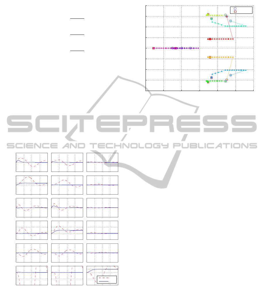
ure 2 shows that decoupling is substantially improved.
The variation of closed-loop poles from their nominal
value is depicted in Figure 3.
−5
0
5
From: θ command
To: q
−5
0
5
To: θ
−5
0
5
To: r
−2
0
2
4
To: ψ
−50
0
50
To: p
0 2 4 6 8
−4
−2
0
2
To: φ
From: ψ command
0 2 4 6 8
From: φ command
0 2 4 6 8
Step Response
Time (seconds)
Amplitude
Initial
Final
Figure 2: Control of a launcher in atmospheric flight. Ini-
tial and final controller obtained respectively by standard
and optimized eigenstructure assignment in the case where
eigenvectors are not structured. Decoupling is improved.
We now wish to design a closed-loop controller to
get decoupling of the modes by choosing some struc-
tural constraints on eigenvectors v
i
. As an illustra-
tion, the eigenvectors v
1
and v
2
are complex conju-
gate to each other and have zero entries in the rows
corresponding to ψ and φ. The eigenvector v
4
is the
−6 −5 −4 −3 −2 −1 0
−2
−1.5
−1
−0.5
0
0.5
1
1.5
2
Real axis
Imaginary axis
Pole map of the process of eigenstructure assignment
Initial poles
final poles
Figure 3: Itineraries of closed-loop poles in optimized
eigenstructure assignment based on Hankel program (5).
complex conjugate of v
3
whose entries relative to θ
and φ are taken as zero. The eigenvectors v
5
and v
6
are complex conjugate and have zero entries in the
rows associated with θ and ψ. For the real modes, the
eigenvectors are chosen as
v
7
= [∗ ∗ 1 ∗ ∗ 0 ∗ 0 ∗ ∗ ∗]
>
,
v
8
= [∗ ∗ 0 ∗ ∗ 1 ∗ 0 ∗ ∗ ∗]
>
,
v
9
= [∗ ∗ 0 ∗ ∗ 0 ∗ 1 ∗ ∗ ∗]
>
.
The controller K
opt
computed by Algorithm 1 gives
kT (P
perf
,K
opt
)k
H
= 0.7360, while the initial con-
troller K
init
obtained by standard assignment has
kT (P
perf
,K
init
)k
H
= 0.7787. Figure 4 illustrates the
improvement in step responses.
7 CONCLUSIONS
We have presented a new approach to partial eigen-
structure assignment in output feedback control,
which is dynamic in the sense that it allows the
eigenelements (λ
i
,v
i
,w
i
) to move in the neighbor-
hood of their nominal elements (λ
0
i
,v
0
i
,w
0
i
) obtained
by standard assignment. This gain of flexibility is
used to optimize closed-loop stability and perfor-
mance. Optimization is based on minimizing the
Hankel norm of the performance channel, as this re-
duces system ringing. The efficiency of the new ap-
proach was demonstrated for control of a launcher in
atmospheric flight.
OptimizedEigenstructureAssignment
313

−1
0
1
From: θ command
To: q
0
1
2
To: θ
−2
0
2
To: r
0
1
2
To: ψ
−1
0
1
To: p
0 2 4 6
0
1
2
To: φ
From: ψ command
0 2 4 6
From: φ command
0 2 4 6
Step Response
Time (seconds)
Amplitude
Initial
Final
Figure 4: Control of a launcher in atmospheric flight. Initial
and final controller obtained respectively by standard and
optimized eigenstructure assignment in the case of struc-
tured eigenvectors.
REFERENCES
Apkarian, P. and Noll, D. (2006). Nonsmooth H
∞
synthesis.
IEEE Trans. Automat. Control, 51(1):71–86.
Burke, J. V. and Overton, M. L. (1994). Differential proper-
ties of the spectral abscissa and the spectral radius for
analytic matrix-valued mappings. Nonlinear Anal.,
23(4):467–488.
Clarke, F. H. (1981). Generalized gradients of Lipschitz
functionals. Adv. in Math., 40(1):52–67.
Clarke, F. H. (1983). Optimization and Nonsmooth Analy-
sis. John Wiley & Sons, Inc., New York.
Gabarrou, M., Alazard, D., and Noll, D. (2013). Design of a
flight control architecture using a non-convex bundle
method. Math. Control Signals Systems, 25(2):257–
290.
Greensite, A. L. (1970). Elements of modern control the-
ory, volume 1 of Control Theory. Spartan Books, New
York.
McLean, D. (1990). Automatic flight control systems. Pren-
tice Hall, London.
Nesterov, Y. (2007). Smoothing technique and its applica-
tions in semidefinite optimization. Math. Program.,
Ser. A, 110(2):245–259.
Noll, D. (2010). Cutting plane oracles to minimize non-
smooth non-convex functions. Set-Valued Var. Anal.,
18(3–4):531–568.
Noll, D. (2012). Convergence of non-smooth descent
methods using the Kurdyka-Łojasiewicz inequality.
Preprint.
Noll, D., Prot, O., and Rondepierre, A. (2008). A prox-
imity control algorithm to minimize nonsmooth and
nonconvex functions. Pac. J. Optim., 4(3):571–604.
Ostrowski, A. M. (1973). Solutions of Equations in Eu-
clidean and Banach Spaces. Academic Press, New
York-London.
Overton, M. L. (1992). Large-scale optimization of eigen-
values. SIAM J. Optim., 2(1):88–120.
Polak, E. (1997). Optimization: Algorithms and Consistent
Approximations, volume 124 of Applied Mathemati-
cal Sciences. Springer-Verlag, New York.
Rockafellar, R. T. and Wets, R. J.-B. (1998). Variational
Analysis. Springer-Verlag, Berlin.
APPENDIX
The numerical data for A and B used in (14) are gath-
ered in the following Table 1.
Table 1: Numerical coefficients at steady state flight point.
Z
w
-0.0162 M
w
0.0022 Y
w
-6e-4 N
q
5e-4
Z
q
87.9 - 88.11 M
q
0.0148 Y
θ
-2.11 N
v
-M
w
Z
θ
-9.48 M
r
-0.0005 Y
v
Z
w
N
r
0.0151
Z
v
0.0006 M
p
0.0042 Y
r
-87.9 N
p
-0.0024
Z
ψ
-2.013 T
q
0.98 Y
ψ
9.47 P
q
0.2078
Z
p
-0.687 T
r
-0.2084 Y
p
-1.965 P
r
0.9782
Z
φ
0.399 L
q
0 Y
φ
1.3272 F
q
0.0704
L
r
0 L
p
-0.0289 L
βr
25.89 F
r
-0.015
Z
βz
10.87 M
βz
4.08 Y
βy
-10.87 N
βy
4.08
ICINCO2013-10thInternationalConferenceonInformaticsinControl,AutomationandRobotics
314