Model-based Analysis of Embedded Systems:

Placing It upon Its Feet Instead of on Its Head

An Outsider’s View

Peter Struss

Comp. Sci. Dept., Tech. Univ. of Munich, Boltzmannstr. 3, 85748 Garching, Germany

Keywords: Embedded Software, Cyber-physical Systems, Software Modeling, Failure-modes-and-effects Analysis,

Functional Safety.

Abstract: This position paper makes a case for a paradigm shift in modeling and analyzing systems with embedded

software for tasks such as testing, fault and safety analysis. We propose a physics-centered rather than

software-centered perspective, based on the argument that the behavior and misbehavior of the physical

system determines the relevant aspects of the embedded software. The implications of such an approach are

illustrated using a case study on failure-modes and effects analysis in the automotive industries.

1 INTRODUCTION

Nobody will doubt that embedded software is a

special class of software. It is characterized as being

a software component (or several ones) that is

integrated in a physical device or plant and

interacting with the physical components of this

overall system. In cyber-physical systems (CPS),

several systems with embedded software interact

physically and/or through communication, which

often results in a dynamic structure and context.

We argue that many tasks in model-based

development and analysis of systems with embedded

software, such as design verification, failure-modes-

and-effects analysis (FMEA), diagnosis, test

generation and testing, cannot be performed

effectively and successfully, unless its specificity,

namely being embedded in the physical system,

dictates the style and content of the model and the

analysis, rather than understanding systems

engineering of CPS just as extending software

engineering to physical systems. “Our modeling and

approach does not distinguish between software and

physical components” is not an advantage, but

indicates a major lack.

Our claim is not only that modeling of physical

systems cannot be done in the style of modeling

software. More than this: the behavior and

modeling of the physical system determines the

way of modeling the software and helps to

simplify and focus it.

In this paper, we motivate our position by

general considerations about CPS and illustrate the

resulting approach, which places the analysis upon

the feet (the physics) instead of on its head (the

software) using a case study in the automotive

industries on failure-modes-an-effects analysis and

functional safety analysis.

2 CYBER-PHYSICAL SYSTEMS

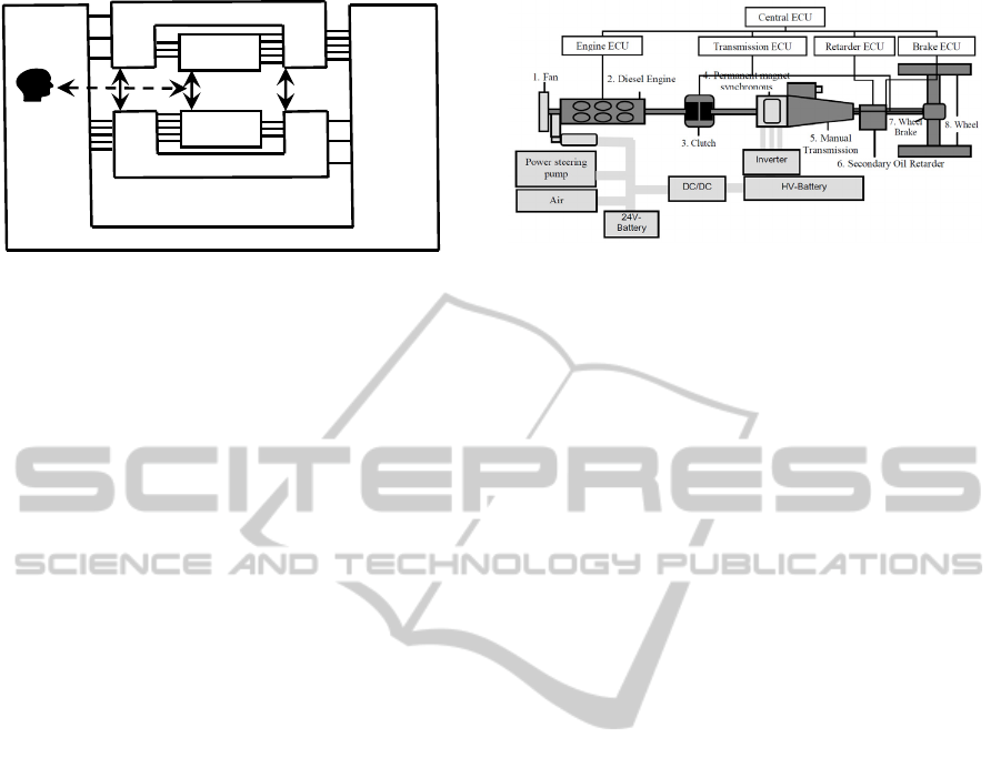
A CPS comprises a number of subsystems, which

are systems composed of physical (mechanical,

electrical, hydraulic, …) components and software

components, whose interaction happens exclusively

through a usually relatively small set of sensor

signals as an input to and actuator signals as an

output of the software component(s) (see Fig. 1).

Different subsystems interact both via connections

between their physical components and via

communication between their software components.

For instance, in a vehicle, the components of the

drive train with their individual ECUs are examples

for such subsystems. At a higher level, the drive

train itself can be considered as a subsystem. The

top-level system is the entire vehicle.

The key issue here is that only the behavior of

the physical system matters. For instance, from the

perspective of safety analysis, it is important to note

284

Struss P..

Model-based Analysis of Embedded Systems: Placing It upon Its Feet Instead of on Its Head - An Outsider’s View.

DOI: 10.5220/0004596102840291

In Proceedings of the 8th International Joint Conference on Software Technologies (ICSOFT-EA-2013), pages 284-291

ISBN: 978-989-8565-68-6

 2013 SCITEPRESS (Science and Technology Publications, Lda.)

SW_x

Physical System_x

SW_y

Physical System_y

Environment

Data

Information

Physical

Interaction

Physical

Interaction

Physical

Interaction

Figure 1: Cyber-physical Systems.

that it is solely the physical system, i.e. the vehicle

(or its physical parts) that interacts with the

environment. The embedded software never

directly interferes with the environment. As a

consequence, hazards, misbehaviors that bear the

potential of damage in the environment, are defined

exclusively at the intersection of the physical

system and the (physical) environment. Whatever

crazy operations may be carried out by the software

– they are never a hazard per se. They may only

cause one via the response of the physical system to

the actuator signals. So far, no computer program

has ever hit a pedestrian.

As an important consequence, buggy software

behavior matters if and only if it may cause the

physical system to create a hazard. Therefore, our

approach moves the (model of the) physical system

into the center and models software – and

especially software faults – solely with regard to the

physical model. As a consequence, the relevant

misbehavior of the physical system helps to simplify

and focus the modeling and analysis of the

embedded software:

 While the inputs to the software (combinations of

sensor values) form an infinite space from the

frog’s perspective of the software, the surrounding

physical system and its context reduce this to the

physically possible subspace (one has to note,

however, that this does not only include the

nominal, but also faulty behavior).

 Furthermore, what is considered a relevant

misbehavior or hazard of the entire system

determines a focus and weight on the analysis of

the software components.

We illustrate the principle of the primacy of the

physical model using a recently performed case

study, which included Failure-modes-and-effects

(FMEA) and safety analysis of the drive train of a

truck. The drive train comprises, besides

mechanical, hydraulic, and electrical components, a

number of Electronic Control Units (ECU) and, thus,

is certainly an instance of the class of systems we

Figure 2: Drive Train Model.

are considering in this paper. The goal of our work

was the complete automation of the analysis based

on a model of the system and its environment. This

goal was accomplished as described in (Dobi et al.,

2013).

We briefly sketch the system and the task in the

following section, present the theoretical

foundations of our solution (section 4) and of

automated FMEA (section 5), and illustrate in

section 6 the central thesis of this paper: the

dominance of the behavior and model of the

physical system over the software behavior and

model. Section 7 extends this to the aspect of

generating (safety) requirements on the embedded

software.

3 A CASE STUDY: SAFETY

ANALYSIS OF A DRIVE TRAIN

Our industrial partner, ITK Engineering AG,

selected a drive train of a truck as the subject of a

case study. Its structure is sketched in Fig. 2. The

main part (in dark gray) comprises the engine, which

produces torque for acceleration, but also for

braking, the clutch, which may interrupt the

propagation of torque, the transmission allowing to

switch between forward and reverse torque (and

idling), the retarder, a braking device that, when

applied, counteracts the rotational motion through a

propeller moving in oil, and the axle with the wheel,

which transforms rotational acceleration into

translational acceleration (and vice versa), and the

wheel brakes. Components are controlled by

specialized ECUs, which communicate with a

central ECU that processes, for instance, the driver

demands. The light-gray components are related to

electrical aspects and are not discussed in this paper.

The industrial partner also supplied us with

documents on exemplary problems and manually

generated safety analysis tables. The core of an entry

in such a table links a component fault (e.g.

Model-basedAnalysisofEmbeddedSystems:PlacingItuponItsFeetInsteadofonItsHead-AnOutsider'sView

285

“erroneous CLOSE command to the clutch”), a

special driving situation (“engine running, vehicle

standing”), and a type of scenario (“vehicle in front

of pedestrian crossing”) with a hazard (“unintended

forward acceleration”) and its impact on the

environment (“injury of persons”). Relevant impacts

are typically hit-ting objects or persons, where,

obviously, the severity is influenced by the type of

object.

4 MODELING FOUNDATIONS

4.1 Physical vs. Software Modeling

At a very high level, the model of a cyber-physical

system may not explicitly distinguish whether its

subsystems of components are software modules or

physical components, and they may be represented

in a uniform way, e.g. as black boxes with some

mapping from inputs to outputs or as transition

systems. Often, these models try to capture the

(intended) function of a system, rather than its entire

possible behavior. For instance, in early phases of

design, it may not yet have been decided whether a

certain subsystem will be realized by software, a

physical system, or a combination of both.

However, when the behavior has to be analyzed

in detail, the different nature of software and

physical components will often require models that

appropriately capture the physical phenomena that

determine system behavior. This is even mandatory

when the consideration of faulty behavior is

involved, as e.g. in diagnosis, testing, or safety

analysis: While the space of bugs in the software

components is created by erroneous (manual or

automated) transformations on the path from

requirements to code (and also inappropriate

requirements), faults of physical components are

exclusively subject to the physical defects, which

often makes it possible to enumerate and model the

relevant fault classes. Moreover, most physical

components, e.g. in electrical, mechanical,

hydraulic, and pneumatic circuits cannot be

modeled by input-output behavior. Even if they

have an intended preferred direction under nominal

system behavior, this may be totally perturbed under

the presence of a fault. Therefore, our approach

presented is based on relational models of the

physical components, which also induces a small set

of generic high-level (fault) models of the software

components.

The characteristics of the models used in our

solution are the following:

 Compositional modeling: models of systems are

obtained through aggregation of models of its

parts, possibly across several layers of hierarchy.

 Component-oriented modeling: the parts are

components, i.e. the building blocks that are

assembled to form the system and determine its

behavior (both physical and software components).

This is due to two reasons. Firstly, component

models can be reused in different system models

just as the components are reused in different

systems. Secondly, components are the entities

that are subject to faults, whose impact needs to be

determined in safety analysis.

 Qualitative behavior models reflect the qualitative

and worst-case nature of the analysis.

 Relational models (as opposed to transition

systems) are chosen to represent these qualitative

behavior descriptions, according to the

considerations above and justified by the

observation that hazards are commonly the result

of a fault in one state of the physical system (rather

than occurring after a sequence of state

transitions).

 Deviation models are used, since faults, hazards,

and impact are characterized as (qualitatively)

distinct from nominal behavior.

In the following, we specify these characteristics

more formally, though in a nutshell (For

introductory material, see e.g. (Struss, 1997),

(Struss, 2008).

4.2 Component-Oriented Modeling

A component type (used to create different

instances) is represented under a structural and a

behavioral perspective:

 It has a number of typed terminals, which can be

shared with other components.

Thus, a system structure is described by as

(COMPS, CONNECTIONS), where COMPS is a set

of (typed) components and CONNECTIONS is a set

of pairs of terminals of equal type belonging to

different components.

 A component C

has a vector v

= (v

) of variables,

comprising parameters and state variables,

which are considered as internal and constant and

changing dynamically, resp., and terminal

variables. The latter are obtained from the

instances of the terminal types, which have a set of

associated variable types.

The CONNECTIONS of a system structure induce a

set VARIABLECONNECTIONS of pairs of

corresponding terminal variables from connected

ICSOFT2013-8thInternationalJointConferenceonSoftwareTechnologies

286

components. Each variable connection introduces a

mapping between the values of the connected

variables: this is usually equality (for signals,

voltage etc.), while for directed variables, such as

torque and current, the sign is flipped.

 A component C

has a set of behavior modes

{mode

)}, where one mode, OK, corresponds to

the nominal behavior of the component and the

other ones denote different defects of the

component.

4.3 Qualitative Modeling

Qualitative models describe component behavior in

terms of variable domains DOM (v

) that are finite.

Besides domains that are considered “naturally”

discrete, such as Boolean for binary signals and

{OPEN, CLOSED} for the state of a clutch, the

domains of continuous variables are obtained by

discretization and are usually finite set of intervals

that reflect the essential distinctions needed for

capturing the relevant aspects of component

behavior:

DOM (v

) = {I

ikm

 m=1, 2, …, n}

4.4 Relational Modeling

The behavior of a component under a particular

behavior mode, mode

), is represented as the set

of qualitative tuples that are possible if this mode is

present, i.e. as a relation

 DOM(v

) =

DOM (v

)  DOM (v

)  ...  DOM (v

) ,

or, in AI terminology, as a constraint (which means

many operations on models introduced in the

following can be realized using techniques of Finite

Constraint Satisfaction).

Each variable connection (v

, v

) introduces a

relation R

capturing the mapping between

domains.

4.5 Compositional Modeling

A model of an aggregate system is not unique, but

dependent on the behavior modes of the

components. A mode assignment MA = {mode

)}

specifies a unique behavior mode for each

component, and a model of the system is obtained as

the (natural) join (as in the relational algebra and

SQL, see (Codd, 1970)) of the mode models:

= R

(1)

4.6 Deviation Models

Some are stated in absolute terms ("zero braking

torque exerted by brake") others are only described

in relative terms ("reduced braking torque produced

by a worn brake"), and so are definitions of hazards:

"reduced deceleration of vehicle". Such models are

meant to capture qualitative deviations from the

nominal behavior, which is the basis for detecting

deviations in the behavior of the entire system.

We use deviation models in the same way as in

(Struss, 2004): the qualitative deviation of a variable

v is defined as

x:= sign(x

act

nom

)

(2)

which captures whether an actual (observed,

assumed, or inferred) value is greater, less or equal

to the nominal value. The latter is the value to be

expected under nominal behavior, technically: the

value implied by the model in which all components

are in OK mode.

Qualitative deviation models can be obtained

from standard models stated in terms of (differential)

equations by canonical transformations, such as

a + b = c  a

⊕

b = c

a * b = c 

a

act

⊗

b)

⊕

act

⊗

a)

⊝

(a

⊗

b) = c,

with the addition, multiplication, and subtraction

operators of interval arithmetic:

⊕

⊗

⊝

5 AUTOMATED FMEA

For both the analysis of hazards (unwanted behavir

of a vehicle) and the overall impact analysis, we

exploit an algorithm that has been used for FMEA

(Picardi et al., 2004), (Struss and Fraracci, 2012).

The algorithm is based on representing not only

behavior models as finite relations (as described in

4.4), but also effects and scenarios. Effects can

naturally be stated as relations E

on system

variables that characterize the relevant aspects of

system behavior, such as (the deviation of) the

acceleration of a vehicle, while a scenario is

typically a relation S

on exogenous variables and

internal states of the system like the position of the

brake pedal (pushed or not) and the vehicle speed.

The algorithm checks the presence of effects for

Model-basedAnalysisofEmbeddedSystems:PlacingItuponItsFeetInsteadofonItsHead-AnOutsider'sView

287

each possible single fault in the system under each

defined scenario. Using the relational representation,

this means that for a mode assignment MA

that

contains exactly one fault mode and OK modes

otherwise, the respective behavior model R

MAi

automatically composed according to (1). Then, for

each scenario S

and each effect E

, it is determined

whether

 

MAi

⋈

)  E

where 

denotes the projection (as used in the

relational algebra) to the variables of E

. The

positive case, i.e. the failure mode is included in

effect, means that the effect will deﬁnitely occur.

Stated in logic, this means that the fault entails the

effect in this scenario.

 

MAi

⋈

)  E

=  .

If the intersection is empty, the effect does not

occur. Logically, the effect is inconsistent with the

fault mode and the scenario.

 Otherwise, the effect possibly occurs, i.e. 

MAi

⋈

) covers both conditions under which the

effect is present and others under which it does not

occur – the effect is consistent with the fault mode

and the scenario.

In our project, we used the FMEA engine of Raz’r

(OCC’M, 2013), which implements this approach to

autmatically generate effects at different levels:

 at the system level, i.e. the entire vehicle, in terms

of unwanted accelration and deceleration of the

truck

 in the interation with the enviroinment, in terms of

collisions with persons and other vehicles and

objects.

6 DRIVE TRAIN MODELS

The components of the drive train determine the

acceleration or deceleration of the vehicle. More

precisely, engine, crank shaft, clutch, gear box,

retarder, and wheel brakes together determine the

torque on the axle, and the wheel in interaction with

the road surface transforms the torque into a

translational acceleration of the entire vehicle – or

not, if the friction between road surface and tire is

low. Things get even more complicated, when the

road has a non-zero slope and gravity adds a force

that accelerates (or decelerates) the vehicle – again,

dependent on friction: with sufficient friction, the

gravity component along the road will add another

torque to the axle (which may be overcome by other

torques), otherwise, it will directly contribute to the

translational acceleration of the vehicle (sliding

downhill).

These considerations indicate that the modeling

task is non-trivial. The issues to be addressed are

 The overall (deviation of the) torque applied

cannot be determined locally, but only as the

combined impact of several components.

 The transformation of torque into an accelerating

force and vice versa

 The modeling of software components and,

especially, software faults, which seems to be in

the complexity class of clearing out the Augean

stables.

We discuss these aspects in the following.

6.1 Physical Components

We use deviation models as outlined in section 4.6.

Faults may introduce non-zero deviations, e.g. the

model of a worn brake would result in a deviating

braking torque, which depends on the direction of

the rotation (static friction)

T

brake

= 

or the applied torque in case of kinetic friction

T

brake

= T

wheel

Models of OK and faulty behavior are stated in

terms of constraints on the deviations. For instance,

a closed clutch simply propagates a deviating torque

coming on the left from the engine to the right

(flipping the sign):



T

right

= -



left

Here, and throughout the paper, most variables have

values from the domain Sign = {-, 0, +}: torques and

forces, T and F, rotational and translational speeds,

 and v. The commands and states explicitly

discussed here have Boolean values {0, 1}.

Space limitations do not permit presenting the

entire model library (see Dobi et al., 2013) for

details). In the following, we try to outline the key

ideas and illustrate them by selected component

models.

The core purpose of the drive train component

models is to determine the (deviation of the) torque

acting on the axle, which determines the (deviation

of the) translational acceleration of the vehicle (if

the road surface permits). As stated above, the

overall torque results from the interaction of all

components, which potentially contribute to it. The

engine can produce a driving torque, the braking

ICSOFT2013-8thInternationalJointConferenceonSoftwareTechnologies

288

elements (wheel brake, retarder, engine) may

generate a torque opposite to the rotation, and the

clutch and transmission may interrupt or reverse the

propagated torque.

Our current model is based on assuming that

there are no cyclic structures among the

mechanically connected components, which is the

case in our application, but certainly also in a much

broader class of systems. The component models

link the torque (deviations) on the right-hand side to

the one on the left-hand side, possibly adding a

torque (deviation) generated by the respective

component. Hence, at each location in the drive-train

model, the (deviations of) torques represent the sum

of all torques collected left of it.

Whenever a terminal component (in our case the

wheel) or a component in a terminal, i.e. open, state

(the clutch and the transmission) is reached, the

arriving torque is the total one for the section left,

and for the open components, the torque on the

right-hand side is zero, as exemplified by the clutch

(state=0 means open):

state=1  T

right



left

state=0  T

total



left



right

= 0.

Determining the deviation models is not as

straightforward, as it may appear, as we will explain

using the model of retarder as an example. If

engaged (state=1), it will generate a torque opposite

to the rotation (zero, if there is no rotation) and add

it to the left-hand one. The base model is obvious:

right



left

 T

brake

state = 1  T

brake

= - 

state = 0  T

brake

= 0 ,

where  denoted addition of signs. The first line

directly translates into a constraint on the deviations:

T

right

= 



left

 T

brake

However, determining T

brake

requires consideration

of how the actual state is related to the nominal one,

which depends on the control command to the

component, and, to complicate matters, not on the

actual command, but the command that

corresponds to the nominal situation. This means

we have to model possibly deviating commands, and

we apply the concept and even the definition of a

deviation also to Boolean variables. For instance, in

the retarder model, state = - means state = 0 (i.e. it

is not engaged) although it should be 1, and state =

+ expresses that it is erroneously engaged. Such

deviations could be caused by retarder faults, e.g.

stuck-engaged. However, in the context of our

analysis, we must consider the possibility that the

commands to the retarder are not the nominal ones

(caused by a software fault or the response of the

correct software to a deviating sensor value). Under

multiple faults, a component fault may even mask

the effect of a wrong command (the retarder stuck

engaged compensates for cmd = -). In the OK

model of the retarder, it does what the command

requests and the deviations of the command and

state (i.e. the real, physical state) are identical:

state = cmd .

For a stuck engaged fault, however, Table 1 captures

the constraint on the deviations:

Table 1. Retarder stuck engaged - Deviation constraint.

cmd



cmd state

1 0 0

0 0 +

0 - 0

1 + +

Here, the third row represents the masking case

mentioned above, while the first one reflects that the

physical state coincides with the command, while in

the second one, it does not.

From state, T

brake

is determined by

T

brake

= -   state,

where  denotes multiplication of signs. This

completes the model of the retarder.

6.2 Software Models

Since the drive train contains a number of ECUs, we

also need to include models of software and its

faults in our library. Remember: all that matters

about software faults is their impact on the physical

system, more precisely, on the controlled actuator.

Deviations in an actuator signal will often cause a

deviating behavior of the respective actuator. If there

is no command to the brakes although the braking

pedal is pushed, then the brakes do not perform as

expected under nominal behavior (and potentially

cause a collision). And if a continuous signal like the

one controlling the amount of injected fuel is too

low, this may result in a reduced acceleration of the

vehicle.

Such deviations in actuator signal can have two

reasons:

 The software works correctly but based on a

deviating input from sensors or other ECUs (e.g. a

wrong measurement of the outside temperature

may lead to an inadequate computation of the

amount of fuel to be injected.

 The software is buggy and therefore produces a

wrong output (e.g. due to a wrong computation of

Model-basedAnalysisofEmbeddedSystems:PlacingItuponItsFeetInsteadofonItsHead-AnOutsider'sView

289

the fuel amount).

This means: the OK model of software functions

needs to capture how deviating input from sensors or

input other ECUs influences potential deviations in

the actuator signals.

For instance, assume that the command to

engage the retarder as an additional braking element

is based on the rotational speed  exceeding a

threshold. In our context, the only interesting aspect

is how the (correct) function propagates a deviation

of a sensor value (or a missing one). Slightly

simplified, this can be stated as

cmd = _s ,

where _s is the sensor signal and cmd is defined

w.r.t. the domain {0, 1} of cmd. If the _s is too low

(high), i.e. deviates negatively (positively) and,

hence, reaches the threshold too early (too late), this

causes the command to be sent too early (too late),

i.e. the command deviates positively (negatively):

 Untimely (or early) command: cmd = +

 Missing (or late) command: cmd = -

These are also the definitions of the only relevant

faults of the software function, regardless of how

they are produced in detail. For instance, the

threshold being too high (low) has the same impact

as the sensor signal being too low (high). However,

for Software FMEA and safety analysis, the detailed

nature of the fault does not matter.

The same applies to continuous actuator signals,

such as the fuel injection, where the faults represent

signal too low and too high, respectively.

This provides evidence for our claim that putting

safety analysis back on its feet and the physical

model in the center, greatly simplifies the modeling

and analysis of the embedded software. In particular,

for the purpose of hazard analysis, we obtain a small

set of reusable software models for our library. Of

course, if we do have a more detailed model of the

software, also the fault models can be more specific.

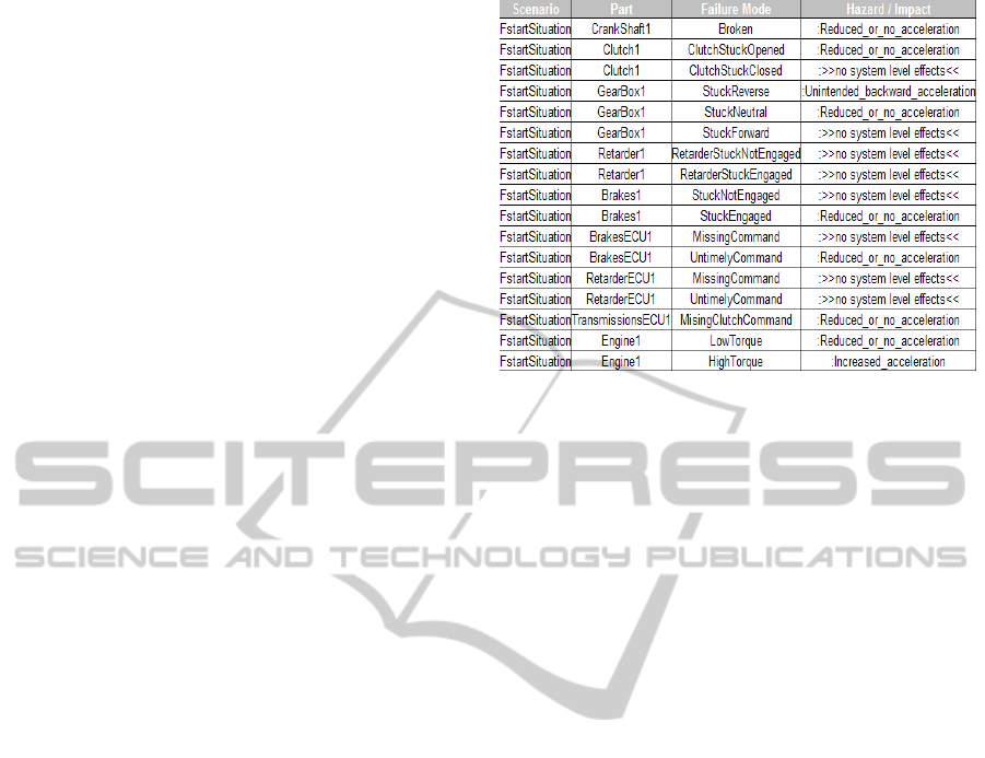
6.3 Results

The automated FMEA generates models of the entire

system with one fault injected at a time and checks

for the effects on the vehicle (“hazards” like

“reduced deceleration”) or on the environment

(collisions). Based on the modeling principles

outlined above, this includes sensor and software

faults. Figure 3 shows an example of the results,

which are presented in (Dobi et al., 2013).

Figure 3: Hazard analysis for “vehicle start”.

7 DERIVING (SAFETY)

REQUIREMENTS

In the work presented above, the models were used

for determining hazards and their impact on the

environment, i.e. for analysis only. However, the

model also forms the basis for the derivation of

safety requirements and, hence, can contribute to re-

design for safety. We illustrate this potential in an

abstract way: First, in the analysis step, a particular

physical scenario, S

, (say, heavy braking on a

slope) is mapped to the input channel of the software

by the physical model, M

, as a set of sensor signals,

or, rather ranges of sensor signals, (pressure, wheel

speeds, etc.),

=

⋈

) ,

where 

denotes the projection to the input channel

of the embedded software.

The software model M

needs to determine the

respective output in terms of actuator signals (e.g. to

the valves controlling the braking)

=

⋈

where 

is the projection to the output channel.

Based on the scenario S

and O

, which is the input

to the physical system, again the physical model M

determines the behavior of the physical system with

respect to its environment:

=

⋈

where 

is the projection to the interface of the

physical system to the environment (e.g. too high

deceleration), which may then, through a context

ICSOFT2013-8thInternationalJointConferenceonSoftwareTechnologies

290

model M

lead to a relevant impact on the

environment.

On this basis, safety requirements for the

embedded software may be determined by back-

propagating a safety requirement on the behavior of

the physical system to the software: avoiding the

impact by avoiding the hazard B

establishes a

revised system response B’

, (e.g. the negation of

). M

infers a required modified software output

in scenario S

O’

=

(B’

⋈

i.e. the requirement on the modified software model

M’

⋈

=

(B’

⋈

or stated in a functional view:

M’

: 

⋈

)  

(B’

⋈

Again, this illustrates the primacy of the physical

perspective, because both the scenario and the

behavior requirement are formulated at the level of

the physical interaction, and the model of the

physical system determines the requirements on the

software.

8 SUMMARY

The case study and its results support our claim that

modeling and model-based analysis of embedded

software is both greatly improved and simplified by

a modeling perspective that focuses on the model of

the physical system.

We successfully applied this approach also in

another case study to automated FMEA of a braking

system (Struss and Fraracci, 2012).

The modeling applied in these case studies

avoids some of the most frequent pitfalls or

inadequacies in modeling physical components in

software and systems engineering, namely

 modeling function instead of behavior, which is

strongly related to

 modeling them in a context-dependent, rather than

generic manner,

 modeling components with input-output behavior,

which is related to

 modeling them using finite state machines instead

of (abstractions of) (differential equations).

The results obtained have triggered interest in

pursuing this line of research. We are currently

preparing a collaborative project involving

automotive companies and academic partners

(representing model-based approaches from AI and

software engineering) that aim at providing tools for

functional safety that are compliant with the

standards and processes. This will require

embedding the analytic part covered here with

higher-level models from design and also feeding

back its results to the process of responding to

severe shortcomings by developing appropriate

safety functions. Steps towards formal foundations

for an integration of the model-based systems and

software engineering technologies will be required

for this.

ACKNOWLEDGEMENTS

I would like to thank our partners from ITK for

providing their domain knowledge and their patience

and Sonila Dobi and Alessandro Fraracci for their

support. Special thanks to Oskar from OCC’M

software for producing a very efficient

implementation of the FMEA algorithm.

REFERENCES

Codd, E. F., 1970. A Relational Model of Data for Large

Shared Data Banks", in Communications of the ACM

Dobi, S., Fraracci, A., Gleirscher, M., Spichkova, M.,

Struss, P., 2013. Model-based Hazard and Impact

Analysis, Tech. Report, TU Munich, Comp. Sci. Dept.

OCC'M Software GmbH, 2011. Raz'r Model Editor

Version 3. Interactive Development Environment for

Model-based Systems. http://www.occm.de/

Picardi, C., Console, L., Berger, F., Breeman, J., Kanakis,

T., Moelands, J., Collas, S., Arbaretier, E., De

Domenico, N., Girardelli, E., Dressler, O., Struss, P.,

Zilbermann, B., 2004. AUTAS: a tool for supporting

FMECA generation in aeronautic systems. In:

Proceedings ECAI-2004 Valencia, Spain, pp. 750-754

Struss,P., 2004. Models of Behavior Deviations in Model-

based Systems. In. Proceeding of ECAI-2004

Valencia, Spain, pp. 883-887.

Struss, P., 1997. Model-based and qualitative reasoning:

An introduction. In: Annals of Mathematics and

Artificial Intelligence 19 (1997) III-IV, Elsevier, pp.

355 - 381, 1997.

Struss, P., 2008. Model-based Problem Solving In: van

Harmelen, F., Lifschitz, V., and Porter, B. (eds.).

Handbook of Knowledge Representation, Elsevier, pp.

395-465

Struss, P., Fraracci, A., 2012. Modeling Hydraulic and

Software Components for Automated FMEA of a

Braking System. In: Dearden, R. and Snooke, N.

(eds.). Proceedings of the 23rd Workshop on the

Principles of Diagnosis. Great Malvern, UK.

Model-basedAnalysisofEmbeddedSystems:PlacingItuponItsFeetInsteadofonItsHead-AnOutsider'sView

291