Design Approaches for Mode Decision in HEVC Encoder

Exploiting Parallelism at CTB Level

Ramakrishna Adireddy and Suyash Ugare

PathPartner Technology Consulting Pvt Ltd, New Thippasandra Main Raod, Bangalore, India

Keywords: Rate-distortion Cost, Coding Tree Block (CTB), Parallel Processing, Mode Decision, Video Quality (VQ).

Abstract: As CPU technology trend is strongly moving towards multi-core architectures, HEVC tried to embrace the

parallel processing trend to possible extent. Hence, HEVC exploits some of the parallel processing

capabilities like tiles, slices and WPP at frame level (Sullivan et al., 2012). Although slices, tiles and WPP

can be used to achieve parallelism, they might end-up degrading either visual quality or compression

efficiency. To address this problem, this paper tries to summarize/exploit the possible parallel processing

capabilities of HEVC at Coding Tree Block (CTB) level with insignificant compromise in video quality and

compression.

1 INTRODUCTION

The emerging video coding standard, High

Efficiency Video Coding (HEVC/H.265) (Bross et

al., 2013), which is also a part of MPEG-H, tries to

achieve up to 50% better compression when

compared to the Advanced Video Coding

(AVC/H.264) standard, while maintaining similar

video quality levels (Sullivan et al., 2012). Although

HEVC uses the same “hybrid” approach and coding

tools similar to prior standards, there are key

differences that enable the enhanced compression.

The higher gains in the compression are the result of

using various high efficiency coding tools available

in HEVC namely - large and variable size coding

blocks, larger and variable size transforms,

Advanced Motion Vector Prediction(AMVP), Merge

prediction blocks and Band Offset Filters & Edge

Offset Filters collectively named as Sample

Adaptive Offset (SAO) filter.

Most of these high efficiency coding tools in the

HEVC encoder are computationally intensive. Also,

since HEVC provides more options to encode a

picture, the challenge at the encoder side is to decide

the “most suitable combination” of the coding tools

for encoding such that both rate and distortion are

minimized to the best possible levels (Bossen et al.,

2012). The “most suitable combination” of blocks

and modes is decided by the mode decision process

of an encoder. Main focus of this paper will be on

understanding the impact of mode decision flow of

an encoder on computatonal complexity and

resulting compression efficiency.

The rest of the paper is organized as follows.

Section 2 briefs the encode mode decision details

that have been considered for the proposed

approaches implementation. In section 3, we brief

the proposed approaches and in section 4, we carry

out comparative study and analysis of proposed two

approaches. Finally, section 5 concludes the paper.

2 OVERVIEW

The ultimate goal of any video coding standard has

been to achieve maximum compression without

compromising on the quality of encoded video.

Mode decision in an encoder is responsible for

making optimal decisions to achieve the said

encoder goals with respect to complexity and video

compression. For a Coded Tree Block (CTB), mode

decision in HEVC encoder comprises of making the

following set of decisions:

 Intra prediction Direction for intra prediction

block(PB)

 Motion Vector (MV) for inter PB

 Merge Decision for Inter PB

 Best Part Mode for Intra CB – 2Nx2N/NxN

 Best Part Mode for Inter CB

2Nx2N/2NxN/Nx2N/NxN/2NxnU/2NxnD/nLx2

N/nRx2N

Adireddy R. and Ugare S..

Design Approaches for Mode Decision in HEVC Encoder - Exploiting Parallelism at CTB Level.

DOI: 10.5220/0004613600230027

In Proceedings of the 10th International Conference on Signal Processing and Multimedia Applications and 10th International Conference on Wireless

Information Networks and Systems (SIGMAP-2013), pages 23-27

ISBN: 978-989-8565-74-7

 2013 SCITEPRESS (Science and Technology Publications, Lda.)

 Intra CB versus Inter CB decision at all depths

 Skip Decision for CB

 Depth of a Coding Block (CB)

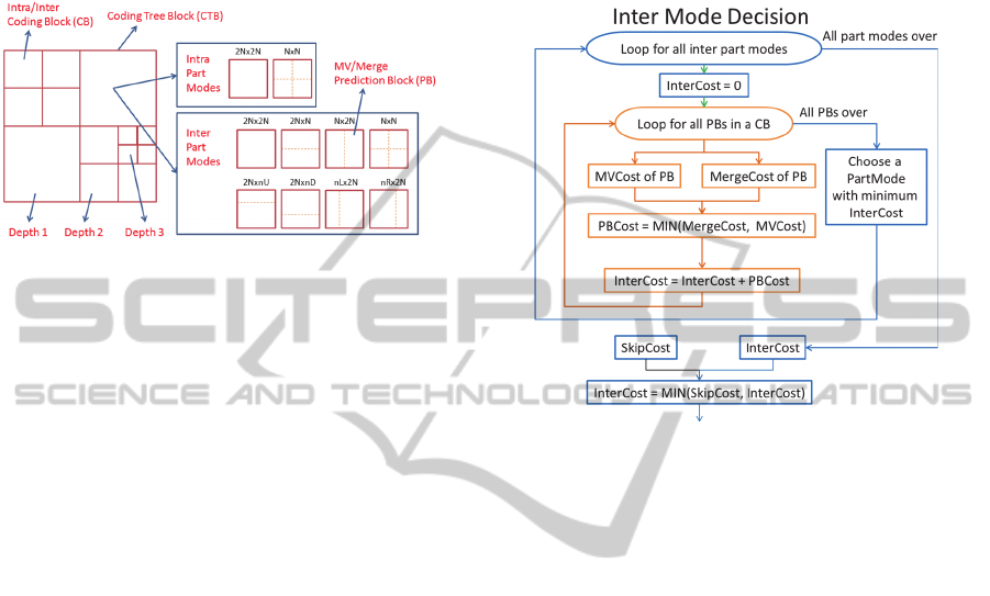
The above decisions may lead to a CTB as shown in

Fig.1.

Figure 1: CTB splitting.

Mathematically, mode decision process has to

minimize cost of the CTB by optimizing rate and

distortion of a CTB so that video compression is

better. According to Lagrangian cost minimization

technique (Sullivan et al., 1998), cost of a block

(CTB/CB/PB) is calculated as

Cost = D + λ* B (1)

where, D is the distortion of a block, B is the bits

required for encoding a block and λ is the

Lagrangian Multiplier whose value majorly depends

on the quantization parameter(QP). Whenever a

decision is to be made between two choices, the

option with lower cost is chosen for coding.

2.1 Inter Mode Decision

For each CB/PB, the process shown in Fig.2 is

applied to take a decision between Inter, Merge and

Skip by comparing their costs. Also, decision is

made to select the best part mode for a CB. Skip can

be coded for a CB only when part mode is equal to

2Nx2N, unlike MV and merge which can be coded

for every part mode. MVCost of a PB is the sum of

MVD bits and prediction error bits. MergeCost of a

PB is the sum of merge index bits and prediction

error bits. SkipCost is the penalty for the distortion

introduced by coding a skip CB.

MV coding cost (MVCost) of a PB is estimated

by Motion Estimation (ME) and Advanced Motion

Vector Prediction (AMVP) technique. Merge cost

(MergeCost) is estimated by using the merge

candidates list. Skip coding decision also depends on

the merge candidate list. Note that, all three

calculations, merge MV, skip MV and AMVP

calculation use the neighbouring coding blocks’ MV

information (Bross et al., 2013). Neighbouring MV

information is used to estimate the coding cost (bits)

of a CB and prediction error is used for estimating

distortion. Output of Fig.2 is Inter Cost of a CB,

featuring a combination of inter and merge PBs or a

skip CB and their corresponding MVs.

Figure 2: Inter coded block mode decision.

Inner loop runs for all PBs in a CB and makes a

decision between Merge PB and Inter PB for all PBs

of a part mode. Outcome of this decision is PBCost,

which is the best of MergeCost and MVCost.

InterCost of a CB is the sum of all PB costs of a

given part mode.

Outer loop runs for all possible part modes and

selects a best part mode having minimum cost. Best

part mode is the one which has minimum cost

according to Eq. 1. After deciding a best part mode

for a CB, its cost is compared with the skip cost to

decide between skip and inter. The final cost of inter

CB is InterCost.

2.2 Intra Mode Decision

Process used for intra CB mode decision is similar to

inter CB mode decision flow and is shown in Fig.3.

There are 35 different intra coding modes for a PB.

The process involves selecting a Rate-Distortion

(RD) optimal part mode for a CB (Choose PartMode

in Fig.3) and an RD optimal intra coding mode for

each PB within a CB (PBCost = Best Intra Mode

Cost in Fig.3). In estimating intra mode cost Most

Probable Mode (MPM) list is used for estimating

coding bits and prediction error is used for

estimating distortion, which depends on the spatial

neighbors of the block. Thus, the output of intra

mode decision process is IntraCost comprising of

SIGMAP2013-InternationalConferenceonSignalProcessingandMultimediaApplications

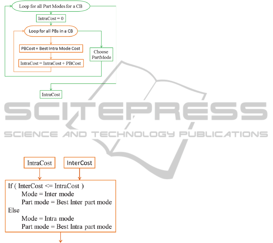
best part mode of the CB and intra mode for each PB

within a CB.

Figure 3: Intra coded block mode decision.

2.3 Intra-Inter Decision

Intra-Inter mode decision process happens for every

CB. Before entering into this process, IntraCost and

InterCost are computed for a CB.

Figure 4: Intra-Inter decision.

InterCost estimate consists of selecting the part

mode of CB and MV/Merge/Skip information of PB.

IntraCost estimate consists of part mode of CB and

selection of intra prediction direction for each PB

within a CB. The decision process involves selecting

the mode with minimum cost as the best mode as

shown in Fig.4.

2.4 Depth Decision

CB can be coded as a single CB or it can be further

split in to a quad tree (4 CBs). Decision has to be

made whether a CB is to split or not. This is done by

comparing the cost of a CB (C) with the sum of

individual sub-CBs cost after the split. If the split

sub-CB cost (C0+C1+C2+C3) is better than the non-

split CB, then the CB is split in to a quad tree. In this

process each CB can be Inter or Intra. Any CB

resulted out of the split CBs can be further split into

in to 4 CBs as seen in Fig.1.

3 APPROACHES TO MODE

DECISION

This section discusses two different approaches for

CTB mode decision. In each approach there are

trade-offs between Video Quality (VQ) and

performance. Each CTB in a frame passes through

the mode decision phase before encoding the H.265

video stream. The two methods discussed below

make an assumption that the encoder processes all

the CTBs one-by-one. Following convention is used

below during discussions - DxCBy refers to Depth x

and CB y, where x = {0, 1, 2, 3} and y = {0, 1, 2 …

64}. For simplicity, in sections 3.1 & 3.2 discussion

is limited to x = {0, 1, 2} and y = {0, 1 …15}

3.1 Method 1 (Ideal VQ)

This method is the one used in reference software,

called the HEVC Test Model (HM10.0, 2013).The

whole process is divided into stages and in each

stage decision is made between two CU depths. The

approach is shown in Fig.5. Each stage is

represented with different color. The numbers within

the CTB or CB indicate the index of a CB at

respective depth. The table shows the processing

method for mode decision.

In the example shown below, 3 depths (D0, D1

and D2) are possible for a CTB of size 32x32. Each

depth has 4

depth

CBs. For each of the CB, at every

depth, Inter Mode Decision, Intra Mode Decision

and Intra-Inter Decision is performed as discussed

earlier in sections 2.1, 2.2 and 2.3 respectively. At

each stage, decision is made whether the CB has to

be split into 4-CBs or it’s to be coded as a single CB

as discussed in Depth Decision.

Stage 1 computes and compares depth-1 cost for

index-0 (D1CB0) and sum of depth-2 cost for

indices 0, 1, 2 and 3 (D2CB0 + D2CB1 + D2CB2 +

D2CB3). Decision is made whether the block is to

be coded as split (depth2) or non-split (depth1)

based on the cost and the resulted best cost is

updated to D1CB0. Stage 1 execution ends here. In

stage 2, similar process is carried out for taking the

split decision for D1CB1. Here cost of depth 1 index

1 (D1CB1) is compared with the sum of cost of

DesignApproachesforModeDecisioninHEVCEncoder-ExploitingParallelismatCTBLevel

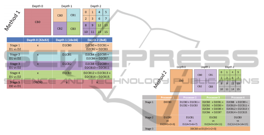
depth 2 indices 4, 5, 6 and 7(D2CB4 + D2CB5 +

D2CB6 + D2CB7). The cost is updated in D1CB1.

Similarly in stage 3 and stage 4 split decisions are

taken and the best cost is updated in D1CB2 and

D1CB3. Once stage 4 is completed, stage 5

compares the cost of depth-0 DOCB0 and total cost

of split CTB (D1CB0 + D1CB1 + D1CB2 +

D1CB3). Note that the cost at depth 1 can be sum of

costs at depth 2. Decision is made whether the depth

0 CB is split or not split.

Figure 5: Different stages in Method-1 flow.

In this method, execution of all stages is

sequential. The sequential flow has an advantage

that the neighbor blocks’ (Left, Top, Top Left, Top

Right and Bottom Left) “accurate” information is

available to the CB being processed. Accurate

neighbor information refers to the to-be-coded mode

information of the neighbors. Since accurate

neighbor information is available to CB, it is

possible to generate exact AMVP list and Merge list

for Inter Mode Decision and MPM list for Intra

Mode Decision, which helps to estimate the bits

required for coding in a more precise manner. Thus,

it is possible to estimate the rate during cost

computation with greater accuracy or rather exactly.

This decision process is able to choose the RD

optimal MVP index, Merge index and MPM index

for inter, merge and intra blocks, respectively.

The approach used in this method is more

suitable for an encoder which has to achieve very

good compression at lower bitrates, which is a high

quality encoder. Also, it is suitable for encoders

which perform the full rate distortion optimization

(RDO) using Lagrangian Optimization or using

Viterbi algorithms. Although this method delivers

good results in compression and quality, this method

is computationally expensive and unfriendly to

multi-processor/parallel-programmable system. This

method’s sequential nature makes each succeeding

stage to wait for the current stage to get completed.

3.2 Method 2 (Performance Friendly)

The approach used in this method is more suitable

for an encoder which has to achieve good

performance (in multi-processor scenario) with a

little compromise on quality. Although, slight

compromise is made w.r.t. neighbor information

availability to the current CB during cost estimation.

Method 2 achieves better performance by taking

advantage of parallel processing. The approach used

in Method 2 is shown in Fig.6.

The example discussed here assumes that a

maximum of 3 depths are allowed and 4 processors

are available for processing. The color in the figure

indicates that the processor on which the block of

data is being processed. The entire mode decision

process is divided into three stages. Each stage is

executed by one or more processors depending on

the stage or on the availability of the processors.

Figure 6: Different stages in Method-2 flow.

In the first stage, each processor operates on one

depth. Processor 1, processor 2, processor 3 and

processor 4 operate on depth 0, depth 1, depth 2

(top) and depth 2 (bottom), respectively. To balance

the processing load, cost computation process in

depth2 is split between processor 3 and processor 4.

At the end of stage 1, the cost of each CB is

available at all depths. All the processors need to

sync after stage 1. In stage 2, decision is made

whether each CB of depth 1 (D1CB0, D1CB1,

D1CB2 and D1CB3) needs to be split to depth 2 or

to be coded at depth 1. The decision process for each

of the 4 CBs can be parallelized across the 4

processors. Again all the processors need to sync

after stage 2 is completed. In stage 3, decision is

made whether the depth 0 is to be coded or the

output of stage 2 is to be retained.

Approach used in method 2 makes good use of

multi-core processing environment. Method two can

be modified easily to work on different number of

cores or even a single core. Since method 2 does not

use accurate neighbor information for estimating the

SIGMAP2013-InternationalConferenceonSignalProcessingandMultimediaApplications

cost, there is a possibility of selecting a suboptimal

mode for coding.

4 COMPARISON OF TWO

APPROACHES

Both the methods have their own pros and cons.

Method 1 is more useful in scenarios where high

quality and greater compression is primary

objective. Method 2 is more useful in scenarios

where parallel-processing is possible and

performance is of prime importance.

In method 1, all CBs at a given depth cannot be

processed in parallel. Each CB has to wait until the

intra-inter decision process and reconstruction of the

previous CB is completed. Intra prediction uses

reconstructed neighbor samples during intra

prediction direction selection. Inter prediction uses

the actual neighbor mode information for

AMVP/Merge/Skip decisions, which helps

achieving better RD cost. In method 2, since coding

blocks are processed in parallel, intra mode decision

process cannot use reconstructed pixels for

prediction. Also intra mode decision and inter mode

decision process does not have access to the

neighbor mode information and have to function

assuming the neighbor mode information for

decisions. Hence the modes selected in method 2 are

with some approximations which affect the

compression efficiency.

Method 1 is more suitable for encoders which

perform full RD during mode decisions as accurate

neighbor information is available to all CBs which

contribute in achieving better compression when

compared to method 2. Although Method 1 tries to

deliver better quality, it cannot take greater

advantage of multi core processing when compared

to Method 2.

5 CONCLUSIONS

In this paper, we proposed a novel method to exploit

the parallelism at CTU level in multi-core/multi-

processor scenario. We described both the traditional

and proposed design approaches for mode decision

and compared them for performance and video

quality/compression. Also, briefed the details of

applications in which each method can be adopted

for better results.

Since the experiment of proposed method is

preliminary, we have only presented the ideas and

approaches to exploit parallelism at the lowest

possible granularity. So, our future work will include

evaluating the performance gain & trade off in

coding quality gain compared to the traditional

approach. As well, future work can consider the

proposed approach in hardware realization.

REFERENCES

B. Bross, W.-J. Han, G. J. Sullivan and T. Wiegand, 2013.

High Efficiency Video Coding (HEVC) text

specification draft 10 (FDIS). In JCT-VC 12

meeting,

Geneva, CH.

G. J. Sullivan, J.-R. Ohm, W.-J. Han and T. Wiegand,

2012. Overview of the High Efficiency Video Coding

(HEVC) Standard. In IEEE Trans. on Circuits and

Systems For Video Technology, vol.22, no.12,

pp.1649-1668, Dec, 2012.

F. Bossen, B. Bross, K. Suhring and D. Flynn, 2012.

HEVC Complexity and Implementation Analysis. In

IEEE Trans. on Circuits and Systems For Video

Technology, vol.22, no.12, pp.1685-1696, Dec, 2012.

G .J. Sullivan, T. Wiegand, 1998. Rate-Distortion

Optimization for Video Compression. In IEEE Signal

Processing Magazine, vol.15, pp.74-90.

HEVC Test Model Ref. software 10.0 (HM10.0), 2013.

Available:https://hevc.hhi.fraunhofer.de/svn/svn_HEV

CSoftware/tags/HM-10.0/

DesignApproachesforModeDecisioninHEVCEncoder-ExploitingParallelismatCTBLevel