MOPED: An Agent-based Model for Peloton Dynamics in Competitive

Cycling

Erick Martins Ratamero

Erasmus Mundus Master in Complex Systems Science,

Ecole Polytechnique, Paris, France

Centre for Analytical Science, University of Warwick, Coventry, U.K.

Keywords:

Agent-based Modelling, Computer Simulation, Peloton Dynamics, Flocking, Emerging Complexity.

Abstract:

MOPED (an acronym for Model of Peloton Dynamics) is a proposed model for peloton dynamics in com-

petitive cycling. Using an agent-based approach, it aims to generate the very complex behaviour observed in

real-life competitive cycling from a collective of agents with very simple rules. Members of a peloton try to

minimize the average energy expenditure by riding behind other cyclists, in a behaviour known as drafting.

Drafting cyclists spend considerably less energy than frontrunners, making many different strategies possible.

We incorporate physiology concepts trying to quantify energy expenditure and recovery in different scenarios.

Starting from a very simple model of identical cyclists, multiple iterations with increasing complexity are pro-

posed, incorporating more and more aspects of the real physics involved in this sport. Finally, we analyse the

results and try to compare them to real-life behaviour to validate the model.

1 INTRODUCTION

Despite the appearance of a purely individual sport

where the strongest tends to win, professional cycling

is actually very strategical. A very simple fact gener-

ates complex behaviours and strategies: the fact that

air resistance dictates how much energy an athlete

spends. The drafting effect, thus, plays a big role on

peloton dynamics. The existence of a peloton itself

can be explained by this effect: energy expenditure

when drafting in a single line is reduced by approxi-

mately 18% at 32km/h, 27% at 40km/h, when drafting

a single rider, and by as much as 39% at 40km/h in a

group of eight riders (McCole et al., 1990).

Emerging from this fact is the behaviour observed

in a real-life cycling race: riders tend to group to-

gether and rotate in front of the peloton, trying to min-

imize the average spent energy. When a group tries

to break away from the pack of riders, the peloton de-

cides either to chase them or let them open a time gap.

If the group is deemed too dangerous, the typical be-

haviour is to chase it, and by having a bigger number

of athletes (and therefore a smaller average energy ex-

penditure for the same speed), they normally succeed

in this task. Only when a breakaway group is con-

sidered harmless enough a gap is established, and the

tired riders from this group are normally caught close

to the ﬁnish line.

Based on contributions (Olds, 1998) (Hoenigman

et al., 2011), we take a mathematical approach try-

ing to quantify energy expenditures based on different

factors as speed, gradient of the terrain, cross-section

area and weight of the cyclist, and speciﬁc physiolog-

ical characteristics of each individual. We regard the

rider basically as a static engine on the bike, and con-

sider the external factors that try to impede motion,

such as drag resistance, rolling resistance and changes

in the potential energy (such as when climbing a hill).

Based on these opposing forces and in physiological

data from professional cyclists, we establish an en-

ergy balance consistent with real-life values.

This is not the ﬁrst agent-based approach for mod-

elling competitive cycling; another work (Hoenigman

et al., 2011) does this quite extensively. However,

their work has a focus on ﬁnal results of a race and

a game-theoretical, best-response model for elaborat-

ing strategies. In this work, we focus not on the ac-

tual results of a race, but rather on simulating the be-

haviour of a peloton during a race, under different cir-

cumstances.

Also, we take the peloton as a complex dynamical

system. We establish general principles and rules for

the behaviour of each agent, roughly based on ﬂock-

ing models already existing (Wilensky, 1998), calcu-

lating cohesive and separating forces for each agent,

so that they stay together as a group, but having spa-

134

Martins Ratamero E..

MOPED: An Agent-based Model for Peloton Dynamics in Competitive Cycling.

DOI: 10.5220/0004617501340143

In Proceedings of the International Congress on Sports Science Research and Technology Support (icSPORTS-2013), pages 134-143

ISBN: 978-989-8565-79-2

 2013 SCITEPRESS (Science and Technology Publications, Lda.)

tial gaps between them. We alter this model so that it

makes sense in the context of this work and observe a

self-organizing pattern emerge, resembling other nat-

ural dynamical systems (Trenchard, 2012).

We develop a model proposal (MOPED - Model

of Peloton Dynamics) for the dynamic behaviour of a

competitive cycling peloton, in an agent-based fash-

ion, based on a small set of basic rules for each agent.

This rules are derived from the mathematical, phys-

iological and dynamical concepts presented, and the

emerging patterns are roughly similar to those ob-

served in real life and in other systems.

Finally, we discuss the results based on data gen-

erated during simulations for many different parame-

ters of the system. Starting from this data, we try to

establish similarities with real-life cycling behaviour

and validate the constructed model. We see this work

as a ﬁrst step to possible further analysis of this sport

via computational simulation in the future, integrat-

ing even more parameters for natural inﬂuence and

speciﬁc behaviour of the agents. As in any complex

dynamical system, it is possible that, via simulation,

we can be able to study much more closely the in-

ﬂuence of isolated parameters in the performance of

each cyclist and of the peloton as a whole.

2 THE MODEL

When constructing our model, we search for differ-

ent kinds of parameters in order to replicate and ex-

tend the real-life behaviour of cyclists in a peloton.

This work proposed an agent-based model for that.

Agent-based models are very well suited for situa-

tions where dynamics emerge from simple interac-

tions between different individuals, or agents (Wool-

ridge and Wooldridge, ).

When realizing an agent-based model, we search

for a set of parameters good enough for simulating the

expected behaviour of the system, but always keeping

in mind that an overcomplicated model becomescom-

putationally infeasible.

In this work, we model agents as cyclists, each of

them with three different kinds of parameters: me-

chanical, physiological and dynamical. Dynamical

parameters are the same for every cyclist, since they

regulate the way a rider behaves inside the peloton:

trying to keep group unity, but steering away from

nearby agents so that as not to cause a crash. We

choose to make mechanical parameters the same for

everyone, for the sake of simplicity. This way, all

cyclists have the same weight and cross-section. It

would be trivial, though, to extend this model to con-

template some variety in these parameters, so as to

accurately describe real cyclists.

Finally, we have physiological parameters. These

regulate the energy balance of each rider. We have

decided that, instead of having identical agents with

identical physical capacities, it would be more inter-

esting to have them normal-distributed around real-

life parameters from professional cyclists. This way,

we expect to see more interesting results, such as the

peloton whittling down during a long climb due to ex-

haustion from lesser riders. In the following sections,

we detail the approach taken for each set of parame-

ters in our model.

2.1 Dynamical Parameters

In this section, we describe the utilized dynamical pa-

rameters for our model; that is, the set of parame-

ters responsible for interaction between agents and the

peloton behaviour. This is a central part in our model,

arguably the most important. A non-desirable choice

of values here leads to unordered behaviour from the

agents, rendering our energy balance equations com-

pletely useless and turning the model away from the

dynamics it expects to simulate.

As a starting point for our dynamics, we take

a simple ﬂocking model (Wilensky, 1998). In this

model, agents are subject to three different kinds of

forces: separating, aligning and cohesive forces. The

separating force is intended to make agents keep a

minimum separation between them, so that they do

not collapse to a single point. This is well-suited to

our model, since cyclists will try to steer away from

other fellow cyclists, to avoid crashes.

We have, then, an aligning force. This force is

applied to each agent to make it follow the direction

from their nearest neighbours. In our case, this seems

a bit out of place. Naturally, in a bicycle race, all com-

petitors are following the same direction, and steering

inside the peloton is a relatively small change in di-

rection. This way, we have decided to model intra-

peloton movement by purely lateral movement, with-

out change of heading direction. There is, then, no

aligning force in place.

Finally, we have a cohesion force. In the ﬂock-

ing model, each agent turns in to become closer to

its ﬂock-mates, making the group a coherent ﬂock.

As we want to simulate a peloton behaviour, it makes

sense to port this kind of force to our model.

In the previous work, the resulting behaviour of

the agents is to move around freely when far from

other agents. However, when approaching other

agents, this group tends to become a coherent ﬂock,

with agents exhibiting similar headings and staying

together, but with some spatial separation between

MOPED:AnAgent-basedModelforPelotonDynamicsinCompetitiveCycling

135

them.

As an improvement on this ﬂocking model, we

take the Swarm Chemistry model (Sayama, 2007).

This time, different sets of agents have different

parameters for cohesive, separating and alignment

forces, making the proportion between those differ-

ent. This makes different sets behave in different

ways, and they tend to stay together in space, even

though they are not coupled together by anything

other than the similarity of their parameters.

From this work, we take the way of calculating

separating and cohesive forces, with minor adjust-

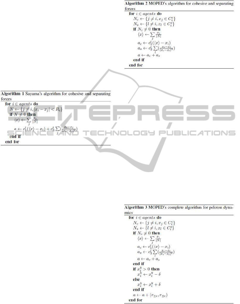
ments for our model. The original pseudo-code from

(Sayama, 2007) is presented as Algorithm 1.

Figure 1: Sayama’s algorithm for cohesive and separating

forces.

With Algorithm 1, we calculate an acceleration for

each agent, based on its relative position to the others.

However, this code calculates it taking into account

any other agent inside R

, a vision radius. This way,

agents actually look all around them when calculating

their new positions. As we are trying to model hu-

man behaviour, it is useful to slightly change this al-

gorithm, so that we only take into account agents that

could possibly be seen by a human, that is, contained

inside a visual cone. We also want to take different

scales of distance when calculating cohesive and sep-

arating forces. Cohesive force should be a long-range

calculation, taking into account pretty much any other

agent in the visual ﬁeld, while separating force is

more local, with only close agents being taken into

account.

Based on these assumptions, we present a new

pseudo-code for these forces, deﬁned here as Algo-

rithm 2.

In Algorithm 2, N

and N

are, respectively, the

neighbourhoods used for the calculation of cohesive

and separating forces. These neighbourhoods are

cones with an aperture angle of 140

, deﬁned to

mimic a human visual cone, and different radii. The

neighbourhood for cohesive force is being used with

a radius of 20m, and the separating one with a radius

of 2m, so that the rider only tries to avoid contact with

other agents in the immediate neighbourhood.

Figure 2: MOPEDs algorithm for cohesive and separating

forces.

A last point to be addressed in this section is some

kind of bias to the center; real cyclists tend to be as

close to the center of the road as possible in the case

where no wind is blowing, so as to avoid danger on

the fringes of the road. A frontrunner would not try

to go too far to one side except if there is a sidewind

blowing, in which case optimal drafting is not directly

behind another rider, but rather in a diagonal. How-

ever, our model does not incorporate sidewinds, and

therefore we want our frontrunners to stay in the mid-

dle of the road. For that, a very small bias is put in

place.

As we also want some variety in the behaviour of

agents, a small, random acceleration is put into place.

With this, we ﬁnish our dynamical model of the pelo-

ton, and then we can move into energetic considera-

tions. A ﬁnal pseudo-code algorithm for this dynami-

cal part would be similar to Algorithm 3.

Figure 3: MOPEDs complete algorithm for peloton dynam-

ics.

As a ﬁnal addendum, we introduce the concept of

active riders: a rider is considered active if he is will-

icSPORTS2013-InternationalCongressonSportsScienceResearchandTechnologySupport

136

ing to cooperate and be the frontrunner of the peloton,

being out of drafting positions in order to protect the

other cyclists. This is modelled by adding a small bias

to the front for active cyclists, as far as they are not

already the frontrunners. This way, the last statement

from the Algorithm 3 would be substituted by what is

presented as Algorithm 4.

Figure 4: Addendum for active cyclists.

We observe that this algorithm, with the right set

of parameters, yields a very life-like behaviour, with

a narrow peloton front giving place to a wider forma-

tion behind, as it can be seen at Figure 5.

Figure 5: View of a simulation of the peloton.

2.2 Energetic Parameters

We will now group together mechanical and physi-

ological parameters, since both sets of parameters af-

fect the energetic balance of the cyclist, making it eas-

ier to analyse them together.

Physiological data about cyclists is abundant; the

literature on how the human body behaves under these

circumstances is extensive and it is not our idea to

redeﬁne anything on this domain, rather than to use

existing results and adjust our model to reﬂect them.

Many mathematical models for competitive cy-

cling exist already. For this model, we will use ele-

ments from (Olds, 1998), who has a validated, well-

behaved set of equations for energy expenditures.

We also use speciﬁc results from (Hoenigman et al.,

2011), who extended Olds’ results and applied it on

an agent-based model, and (Martin et al., 1998) for

the potential-energy equation. By taking an agent-

based approach and simulating both peloton dynam-

ics and energy expenditures, we believe it is possible

to have a more complete model and to have simula-

tions that yield results closer to real life.

Our ﬁrst point is to calculate the drafting coefﬁ-

cient, that is, a correction factor relating the air resis-

tance when drafting and when not drafting. (KYLE,

1979) measured this coefﬁcient experimentally and

afﬁrms that the reduction in air resistance diminishes

when wheel spacing increases. This is a fairly intu-

itive result. He mentions that this reduction obeyed a

second-order polynomial, but he does not present the

equation. (Olds, 1998) reconstructs the equation from

the graphical data, arriving at

dra ft

= 0.62− 0.0104d

+ 0.0452d

(1)

where d

is the wheel spacing (in meters) between

the bicycle and the preceding rider, and CF

dra ft

is the

correction coefﬁcient. However, eq. 1 can be ap-

plied only when drafting happens in a paceline, that

is, when riders are exactly behind one another. In

a peloton, drafting occur also in other ways; riders

in a diagonal have a ”comet’s tail” effect, with draft-

ing bonuses decreasing when the rider behind moves

backwards or sideways. There is no extensive study

of drafting coefﬁcients when a cyclist is not directly

behind another one, as there is no study about draft-

ing multiple riders; we only know that drafting behind

multiple riders is more beneﬁcial than behind only

one (McCole et al., 1990). In this situation, we have

decided to assign weights depending on the angle of

view to the preceding rider. Riders inside a 10

cone

have weight 1; riders inside a 50

, 0.3, and the re-

maining riders inside a 90

cone have a weight of 0.1.

It is important to notice that drafting beneﬁts are neg-

ligible in a distance over 3m, and therefore we limit

our calculations to this radius.

Having calculated CF

dra ft

, we can now go on to

the power equations. As we are using a scale of one

iteration per second of simulation, there is no need

to account for the difference between power and en-

ergy: they are numerically the same. From (Hoenig-

man et al., 2011), we have the following equations:

air

= kCF

dra ft

(2)

roll

= C

g(M + Mb)v (3)

On eq. 2, k is a lumped constant for aerodynamic

drag, dependant, between other things, on the cross-

section area of the cyclist. This constant is generally

reported with the value 0.185 kg/m, and we are fol-

lowing this value. Of course, v is wind speed (and,

as we are considering only a situation without wind,

is equal to ground speed). On eq. 3, C

is a lumped

constant for all frictional losses on a bike, and is gen-

erally reported with a value of 0.0053. Of course, g

is the usual gravitational constant (9.81 m/s

). The

variables M and M

represent, respectively, the mass

of the cyclist and of the bicycle. On this model, we are

using values of 63kg and 7kg, respectively, for these

variables, without any variation between cyclists.

MOPED:AnAgent-basedModelforPelotonDynamicsinCompetitiveCycling

137

These equations are enough for modelling the en-

ergy expenditure of a cyclist in a ﬂat, non-windy situ-

ation. However, we want to model also the behaviour

of the peloton in uphills and downhills, and therefore

we need an extra equation for that. (Martin et al.,

1998) present this equation, for grades up to 10%

(where we consider sin(arctan(G

)) = G

) :

= G

g(M + Mb)v (4)

and, therefore, we can introduce this on eq. 3, ob-

taining the following:

roll+PE

= (C

+ G

)g(M + Mb)v (5)

and a total energy expense of:

= E

= (C

+ G

)g(M + Mb)v+ kCF

dra ft

(6)

But this is only taking into account the energy ex-

penditure. We need to model how the cyclists react

to this and how much energy they can spend without

exhausting themselves. For that, we will introduce

the concept of lactate or anaerobic threshold, very

well-known in any endurance sport. Roughly speak-

ing, the lactate threshold is the power output an ath-

lete is capable of without accumulating lactic acid in

his muscles, that is, without getting tired (Vogt et al.,

2006). In this model, we will assess how tired a rider

is through a simple ”energy-left” variable, so that, at

lactate threshold, the value of this variable is roughly

unchanged.

As presented in (Hoenigman et al., 2011), a speed

of 0.7S

is slightly under the lactate threshold, where

is the speed at which a rider can travel at his Max

power output. The Max

represents the 10-minute

maximum power a rider can generate, and is gener-

ally regarded as an indicator of a rider’s skill level.

We are using, as in that work, a mean value for Max

µ = 7.1W/kg. That represents, for a rider with 63kg,

a Max

of approximately 450W. This is equivalent,

on ﬂat ground, to S

= 12.96m/s. Therefore, 0.7S

approximately 9m/s, and this should be slightly under

lactate threshold. Finally, we take 10m/s as a repre-

sentative value for this threshold, and set a ”recovery”

variable, normally distributed with µ = 225W, that

will be deduced from the actual spent energy. Only

an energy expenditure over this limit will make the

rider grow tired.

We are still faced with the challenge of determin-

ing how long does it take for a rider over his anaer-

obic threshold to be exhausted. For that, we will use

the concept of time to exhaustion (T

lim

), as deﬁned in

(Olds, 1998). The deﬁning equation for T

lim

ln(T

lim

) = −6.351ln( fVO

max

) + 2.478 (7)

In this equation, fVO

max

is the fraction of the

max

(maximum oxygen consumption) being used.

We can substitute that for Max

generating then:

ln(T

lim

) = −6.351ln(

tot

Max

) + 2.478 (8)

For establishing which would be the initial value

of ”energy-left” to each rider, we decided to take an

average situation: a sole rider at 45km/h (or 12m/s).

From that, with our typical Max

of 450W, we cal-

culate which would be the time to exhaustion. From

there, considering our average recovery of 225W, we

calculated how much reserves a cyclist should have at

the beginning of the simulation to achieve this typi-

cal time to exhaustion, arriving at the value of 760kJ.

With that, our modelling of the energy expenditure is

ﬁnished.

2.3 An Overview of the Model

We have presented the two parts of the model: the

dynamicalparameters and equations and the energetic

parameters and equations. Now, we present how these

two parts are interconnected.

It is clear that the position of an athlete inside

the peloton greatly affects his energy balance: if a

rider spends the whole time in front of the peloton,

he will certainly use more energy than another one

sitting safely in the middle of the group. This way,

the dynamical parameters and equations are inﬂuen-

tial on the energy balance. On the other hand, in our

model, the energy balance is, usually, not relevant for

the positioning of the cyclist: position calculation de-

pends only on neighbouring agents. However, when

the cyclist becomes tired, this is then relevant to his

position. We have postulated that a rider with less

than 100kJ of energy left is declared ”exhausted”. An

exhausted rider has a backward bias and is effectively

slower than the peloton average. This way, he tends to

hang at the back of the peloton, eventually letting the

group go altogether. A rider with 0 energy left quits

the peloton altogether. In our model, he is positioned

in the leftmost coordinate and becomes even slower.

However, if he can somehow recover energy enough

to get out of this condition altogether, he will rejoin

the peloton. We present ﬁgure 6, a small, schematic

ﬂowchart representing the relation between the two

”sides” of our model.

3 RESULTS

In the following section, we summarize the results ob-

tained from the simulations using MOPED. These are

icSPORTS2013-InternationalCongressonSportsScienceResearchandTechnologySupport

138

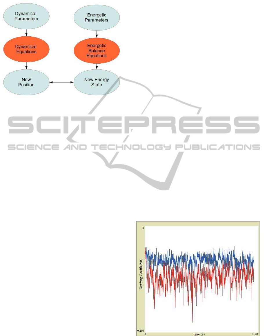
Figure 6: Schematic diagram showing the relation between

parts of the model.

divided between general behaviour, dynamical and

energetic results, for clarity purposes.

3.1 General Behaviour

In general, the emerging complex behaviour from the

agents is very promising; riders rotate back when they

feel they are under the average energy of the pelo-

ton. The peloton itself conforms to the general form

of real-life pelotons, with a very narrow front (usually

a 3-5 long single line of riders) and a widening proﬁle

as we look backwards.

We rapidly see a convection dynamic settling in.

Riders at the back of the peloton wishing to move

forwards take the sides and dash forwards, since the

middle is cluttered with cyclists and going through is

virtually impossible. When they get to the front, they

normally settle down in the center of the road, and as

they stay there other riders coming from the back start

to overtake them. This way, the general dynamics

is: forward-moving cyclists take the sides, backward-

moving cyclists stay in the middle. Of course, to

move forwards through the sides, the athletes end up

spending more energy than those in the center of the

peloton.

(Trenchard, 2012) compares this dynamics to a

convection roll, dissipative dynamic, with ”warming”

riders in the peripheries and ”cooling” riders in the

middle. He then presents other natural systems with

similar dynamics, such as Rayleigh-Bernard cells and

penguin huddle rotations, and hints that this is the way

for achieving optimal energy dissipation in the whole

system. Even though our model does not take any en-

ergy considerations into account for the dynamics, we

still establish similar patterns, which is quite interest-

ing.

Independently of the number of active cyclists

chosen, they rapidly take over the head of the pelo-

ton. Even though not all active agents gather at the

front of the peloton at a single time, most of the time

the frontrunner will be an active cyclist.

When a sustained effort is maintained, cyclists

start to get exhausted and a sizeable group soon forms

at the back of the peloton. Not much after, the ﬁrst

spent cyclists start to appear, giving up on the pelo-

ton. If this effort is maintained for long enough, only

the strongest riders stay in the peloton, with all the

rest giving up. This is consistent with long climbs in

professional races, where the front group is normally

smaller than ten cyclists. Also as in real life cycling,

a long descent after a climb has the effect of bringing

lots of cyclists back to the peloton, as they recover

energy.

3.2 Dynamical Parameters

Most of the results about the dynamics are difﬁcult

to quantify. As commented in the section above, the

general behaviour of the peloton seems coherent with

real life, and furthermore, coherent with an optimal

energy dissipation.

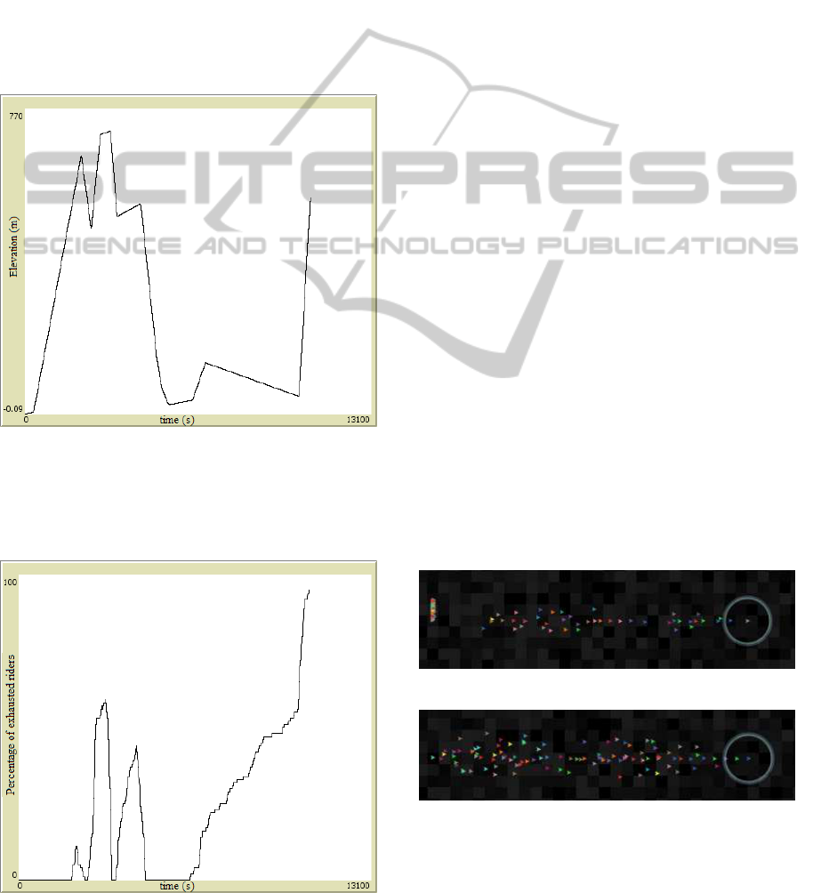
As an addendum, we can show graphically the

convection dynamics. On ﬁgure 7, we have a graph

of average draft coefﬁcient for agents moving forward

(blue) and backward (red). It is clear that, on average,

forward-moving cyclists on the periphery will have

less opportunities to draft behind another cyclists, and

the opposite happens with the central, backward mov-

ing agents.

Figure 7: Temporal distribution of draft coefﬁcient for

backward and forward-moving agents.

MOPED:AnAgent-basedModelforPelotonDynamicsinCompetitiveCycling

139

3.3 Energetic Parameters

At ﬁrst, for illustrating which kind of behaviour our

model generates, we start with an example. We sub-

mit 100 agents to a 3-hour race at a constant speed

of 45km/h. Of course this speed is too high for up-

hill parts, making them spend much more energy than

humanly possible, but we are only interested in the

qualitative behaviour that exhaustion generates. We

generate a proﬁle for the race plotting the elevation at

each time. As we are at constant speed, it is the same

as plotting elevation per distance. The generated pro-

ﬁle is represented on ﬁgure 8.

Figure 8: Temporal proﬁle of our test race.

Subjecting our cyclists to this proﬁle, we generate

then a graph illustrating the amount of exhausted rid-

ers at any given time. The plot is shown as ﬁgure 9.

Figure 9: Exhausted riders (out of 100) at any given time.

We can now establish correlations between both

plots. In the very long initial uphill, relatively few

riders were exhausted. That is, of course, because at

the beginning of the race, every athlete is still fresh.

A slight downhill follows, enough to recover all cy-

clists. However, a second, steepest uphill follows, and

this time the exhaustion is much bigger in the pelo-

ton. Even during the shallow part close to the sum-

mit, the number of exhausted riders is still increasing

considerably. Another downhill follows and, again,

it is enough to recover all riders. Now, a short, not

too steep climb is presented, and the result is a big in-

crease again in exhaustion, this time much more due

to the accumulation of climbs than because of the dif-

ﬁculty of this one. A very long downhill is next, and

of course all riders arrive down there in conditions. A

false-ﬂat (very shallow gradient) do not break them,

but as soon as the road gets steeper exhaustion in-

creases. Even a long, slight downhill after the climb is

not enough to recover, and exhaustion keeps increas-

ing even during this part. Finally, a relatively short,

but very steep climb to ﬁnish the race. This time, only

the very best stay in the front group at the top.

The whole behaviour of the peloton described on

the paragraph above will certainly sound familiar for

anyone who already watched a mountain stage in a

professional cycling race. The patterns are quite sim-

ilar, even if not identical, which indicates that the en-

ergy balance of the model is sound.

As a visual representation of what was described

here, we present ﬁgures 10 and 11. Figure 10 shows

what the peloton looks like at the summit of a long

climb. You can see a relatively small group of 14 rid-

ers in front, followed by a bigger group barely hang-

ing at the back, and many agents already at the left-

most coordinate, representing they have no more en-

ergy.

Figure 10: Peloton at the top of a climb.

Figure 11: Peloton during the descent.

As a comparison, ﬁgure 11 shows the peloton dur-

ing the descent, when the lesser riders havealready re-

covered. You can see the peloton shape is still longest

than normal due to the fact that the back riders are

icSPORTS2013-InternationalCongressonSportsScienceResearchandTechnologySupport

140

still coming back, but there are no more riders with

no energy left and the group is uniﬁed again.

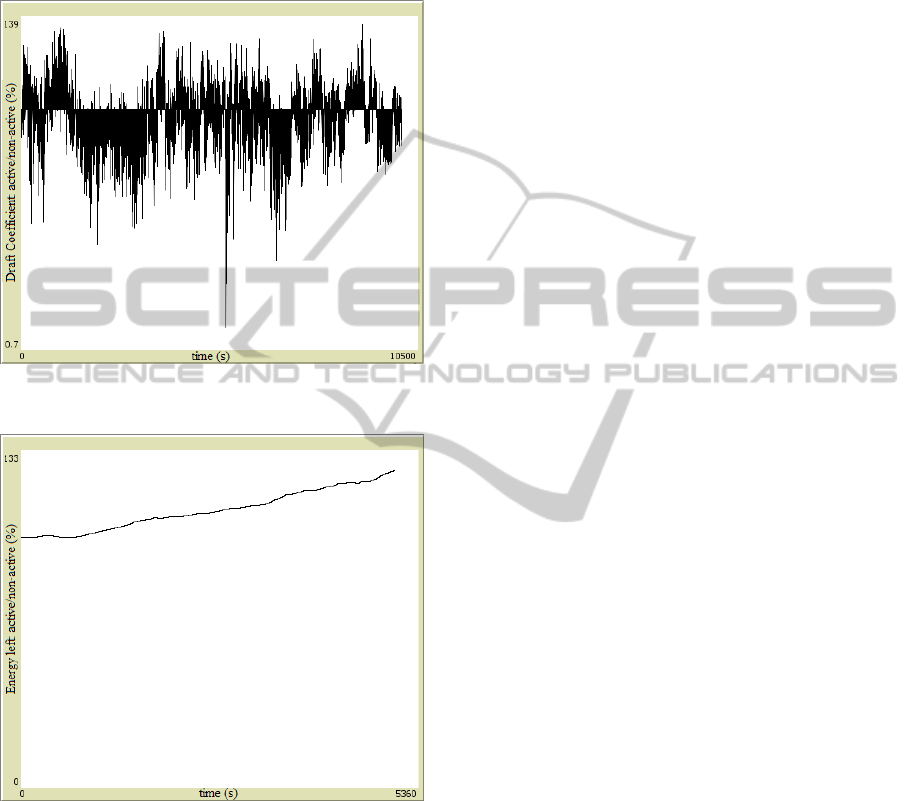
Finally, we present an interesting, counter-

intuitive result derived from the model. We start by

drawing, at ﬁgure 12, the average draft coefﬁcient for

active riders (considering 20 out 100 to be active rid-

ers) compared to the average draft coefﬁcient of non-

active ones.

Figure 12: Draft coefﬁcient of active riders, as a percentage

of DC of non-active riders.

The horizontal reference level is 100%, which would

mean that, on average, active and non-active riders

have similar draft coefﬁcients. However, that is not

what the graph shows: even if it is not that easy to

see on this plot, active riders have signiﬁcantly lower

draft coefﬁcients, which means they spend less en-

ergy. To conﬁrm that, we plot a quocient between av-

erage energy for active and non-active cyclists, and,

even though it starts at 1 as expected, it undoubtedly

increases with time, indicating active riders are, in-

deed, spending less energy on average. This plot is

presented as ﬁgure 13.

This result is surprising, but there are reasons

for it: active riders spend more time on the well-

organized, single line part of the peloton. This way,

they have constantly medium-to-lowdraft coefﬁcients

in these positions. Even if they do have to go to the

front more frequently than non-active riders, this if

offset by the fact that they are consistently drafting

some other cyclists. Non-active riders spend more

time in the convection-like part of the peloton, con-

stantly going back and forth and spending consider-

able amount of time in non-drafting positions at the

periphery of the peloton. Besides that, with much

more movement inside the peloton, they are not guar-

anteed to have another rider right in front of them at

Figure 13: Quocient of energy left between active and non-

active cyclists.

all times, as someone in the single-line part of the

peloton does. This way, their draft coefﬁcient is much

more subject to variations.

This can also be shown by ﬁgure 14, where we

plot a quocient between average neighbourhood size

for active and non-active agents. At the beginning,

when the active agents are still organizingthemselves,

the plot goes under and over 1, but it quickly settles

under 1 as soon as the active riders organize them-

selves. This shows that they are getting smaller draft

coefﬁcients in spite of drafting less cyclists, which is

coherent with the idea that they spend more time ex-

actly behind another cyclist.

Figure 14: Average size of active-agent neighborhood com-

pared to nonactive agents.

All results above are calculated with 20 active rid-

ers out of 100. We may wish to look at different

MOPED:AnAgent-basedModelforPelotonDynamicsinCompetitiveCycling

141

numbers to see if there is any qualitative difference

on these results. This way, we present, on ﬁgures 15

and 16, analogous plots to those at ﬁgures 12 and 13,

but this time calculated for only 5 active agents out of

100.

Figure 15: Draft coefﬁcient of active riders, as a percentage

of DC of non-active riders - 5 active riders.

Figure 16: Quocient of energy left between active and non-

active cyclists - 5 active riders.

It is clear that the qualitative behaviour is exactly the

same, independently of the quantity of active agents.

4 DISCUSSION

This work presents a model for peloton dynamics in

competitive cycling, using an agent-based approach.

Based on a few simple rules for dynamics and energy

balance, we derived a rather complex pattern of con-

vection in the peloton, and coherent results in terms

of energy. Some interesting, counter-intuitive results

arised from the proposed model.

The result where active cyclists spent less energy

than non-active ones does not conform to general

knowledge in cycling, and it shows that there is room

for improvement and calibration in the model. For in-

stance, when moving around, agents do not look for

favourable positions in terms of drafting possibilities,

and the lack of data for drafting in diagonal positions

and behind multiple cyclists hinder the accuracy of

energy distributions.

Besides that, we do not account for many real-life

factors that affect competitive cyclists. An example is

wind, a factor that has major impact in many profes-

sional races. Frontal wind can be modelled as a dif-

ference in speed for the aerodynamical factor in our

energy expenditure equation, but sidewinds require a

whole new approach that was not within the scope of

this work. Of course, there is a different dimension

of cycling that was also not modelled here: the strate-

gic part. ”Intelligent” agents, who know what their

best response to the circumstances of a race is, could

create breakaways, become active or non-active mid-

way during a race, save as much energy as possible

for a ﬁnal sprint. This is certainly feasible as a future

model.

This is probably the ﬁrst time an agent-based ap-

proach is used to try and simulate large-scale cycling

peloton dynamics. Another work (Hoenigman et al.,

2011) take a similar approach, using an agent-based

model to simulate results of cyclingraces. Manyideas

between this work and their work are similar; in spe-

cial, the energy balance is probably quite similar, even

though they do not model uphills and downhills and

this work takes a different approach for modelling the

time to exhaustion of a cyclist. However, their fo-

cus is on obtaining ﬁnal results of the races, while we

want to simulate the dynamics of a peloton during the

race. A different work (Trenchard, 2012) makes some

proto-simulations of pelotons with drafting, looking

for hysteresis on phase transitions. In spite of pre-

senting interesting results, his model is not interested

in simulating the complex dynamics of a peloton, but

only in illustrating a concept.

As the ﬁrst work to explore simulation of such a

complex system as a cycling peloton, we do not ex-

pect this to be a complete work in any way, but rather

to be a ﬁrst step on exploring this fascinating phe-

nomenon of collective behaviour. The results pre-

sented are certainly promising and show that a more

complete model of this system is feasible and can

even show similarities with other natural systems.

icSPORTS2013-InternationalCongressonSportsScienceResearchandTechnologySupport

142

ACKNOWLEDGEMENTS

Many thanks to Prof. Ren´e Doursat (Institut des

Syst`emes Complexes Paris

Ile-de-France) for the

teachings about agent-based models and for support-

ing his students’ ideas. To James Newling, many

thanks for the insightful discussions during the devel-

opment of the model. This work was supported by an

Erasmus Mundus Masters scholarship.

REFERENCES

Hoenigman, R., Bradley, E., and Lim, A. (2011). Cooper-

ation in bike racing when to work together and when

to go it alone. Complexity, 17(2):39–44.

KYLE, C. R. (1979). Reduction of wind resistance and

power output of racing cyclists and runners travelling

in groups. Ergonomics, 22(4):387–397.

Martin, J. C., Milliken, D. L., Cobb, J. E., McFadden, K. L.,

and Coggan, A. R. (1998). Validation of a mathemat-

ical model for road cycling power. Journal of Applied

Biomechanics, 14:276–291.

McCole, S., Claney, K., Conte, J.-C., Anderson, R., and

Hagberg, J. (1990). Energy expenditure during bicy-

cling. Journal of Applied Physiology, 68(2):748–753.

Olds, T. (1998). The mathematics of breaking away and

chasing in cycling. European journal of applied phys-

iology and occupational physiology, 77(6):492–497.

Sayama, H. (2007). Decentralized control and interactive

design methods for large-scale heterogeneous self-

organizing swarms. In Advances in Artiﬁcial Life,

pages 675–684. Springer.

Trenchard, H. (2012). The complex dynamics of bicycle

pelotons. arXiv preprint arXiv:1206.0816.

Vogt, S., Heinrich, L., Schumacher, Y. O., Blum, A.,

Roecker, K., Dickhuth, H., and Schmid, A. (2006).

Power output during stage racing in professional road

cycling. Medicine and science in sports and exercise,

38(1):147.

Wilensky, U. (1998). Netlogo ﬂocking model. Center for

Connected Learning and Computer-Based Modeling,

Northwestern University, Evanston, IL.

Woolridge, M. and Wooldridge, M. Introduction to multia-

gent systems. 2001.

MOPED:AnAgent-basedModelforPelotonDynamicsinCompetitiveCycling

143